PSAL is a SIO-CalCOFI-authored salinity data acquisition program that interfaces with the Guildline Portasal. It can import salt sample base files generated for each station by CESL. A serial data link between the Portasal and data acquistion Windows PC allows PSal to record average conductivity readings, calculate salinities then compare them to CTD salinities.

BASICS

PSAL has three stages: initialization, where the instrument parameters are checked and calibrated to the standard value; sample running, where one or more stations samples are run; end standard, where a final standard or set of standards are run to calculate drift. During the sample running stage, PSAL can preload a salt base files generated by the CESL Sample Logger (ie salt001, salt002...). These base files may contain CTD salts for comparisons which allows a higher degree of preliminary QC.

To begin, press [START], if serial communications between the Portasal & PC handshake correctly, the Comm Status "light" will turn from red to green. An initialization screen will pop-up describing steps required to initialize the machine: check bath temperature; flush cell with standard several times; check Reference reading; check Zero. Once completed, click [OK] to move onto the Load Sub1 step where the Portasal will be calibrated to match the standard or Sub1 value.

Note: Calibrate Sub is done at the beginning of the cruise. Using IAPSO standard water, the Portasal is initialized. Several runs of substandard water are read as samples. The average will become the "Sub1" value for the cruise. IAPSO & Wolga standards are run every other day to calculate any drift in the Sub1 sub-standard.

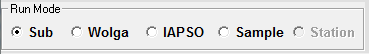
Once the Sub1 is calibrated, it is run at the beginning and end of each session. PSAL will prompt the user to load station samples after the first SUB1. If IAPSO or Wolga standards are to be run, they can be selected by single-clicking the appropriate Run-Mode option.

PSAL expects chronological file numbering - salt001 salt002 salt003 and up to 100 samples (4 full stations) can be run during a session but it is recommended that no more than three stations (~72 samples) be run between Sub1 standards.

PSAL's Current Average box displays a running 5-reading average of the sample. Once saved, subsequent readings must agree with a previous reading within the Agreement Criteria (0.00003 for standards & 0.00004 for samples). During the sample runs, the blue instructions box will prompt the analyst on what should be done next. If the analyst is unable to get two readings to agree within the criteria, he/she can press <F2> and manually pick the best conductivity readings.

SETUP

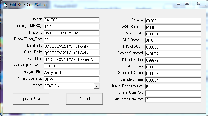
All PSAL settings are configured in the C:\PSAL\psal.cfg file. Data and output filepaths are preset here as well as standard & substandard values, & com port settings.
Two serial ports are typically used: one for the Portasal and a second for the thermometer. The Portasal is installed on com 1, and the thermometer is installed using a usb to serial adapter on com 2 (or whatever is assigned). A printer is often attached directly to the Portasal PC so hardcopies can be printed after the session. Please note that if a printer is unavailable, uncheck the Print Hardcopy option under the Run Info tab.

Tips:

If PSal should crash for any reason, a run can be reloaded by using the [Import Run] option on the Sta Info form or pressing <F6> on the main form and importing the backup csv. The analyst will be prompted to continue the run, run the next station, or save/print.

If the analyst finds themselves out-of-sync with the sample number there are a couple options: if a sample has been run out of order, edit the sample number (Smp) & niskin # (Nis) to match the sample run. Sometimes sample bottles are returned to the sample case out of order and may be run reversed order. This is not a problem unless not noticed. If an incorrect bottle is discovered before the final read, the sample may be swapped with the correct sample and [Restart Sample] pressed to restart the sample read process.
 

Basic Troubleshooting Guide for SIO-CalCOFI's Program Network

Connection to Network & Data Server Directories

• All SIO-CalCOFI programs are designed to be on a common network and the data server (\\seaserv2\data) drive mapped as Q: (or other available letter; set individual program cfg files to the chosen letter). If networking is unavailable, all programs can operate locally by setting drive paths to local letters (ie C:\CODES\2014\1411\...). Base files generated by CESL may be "sneaker-netted" by flash drive - map the datapath to the flash drive (ie F:\Codes\2014\1411\...). Be sure to unmount the flash drive before removing it from the source PC.
• Expected data directory structure: Q:\CODES\YYYY\YYMM\ (ie Q:\CODES\2014\1411\). Subdirectories expected:
  • ..\1411\CHL\
  • ..\1411\CSV\ and ..\1411\CSV\BAK\
  • ..\1411\CTD\  - requires a readme.txt file in order to copy zip files; file content is unimportant but its presence is needed for the zip command to work
  • ..\1411\EVENTS\  - currpos.csv (GPS or MET position), eventnumber.txt (event number), orderocc.txt (station number)
  • ..\1411\LOGS\  - sample log location: CTDBackup-generated base sample log file 1411001.log, 1411002.log... which are loaded into CESL which generates 1411001.slog, 1411002.slog...
  • ..\1411\MAPS\ - location of preliminary contour maps that are generated from CTD mrk or asc files by DECODR
  • ..\1411\MRK\  - secondary location of CTD mrk, hdr, nav, hex, xmlcon files
  • ..\1411\NUT\  - nutrient data dir; data & run files must be copied by the nutrient analyst to the data server using ztree or filesync
  • ..\1411\O2\  - oxygen data dir; data & run files must be copied by the oxygen analyst to the data server using ztree or filesync
  • ..\1411\PROCESS\  - processing log dir; logs for each processing step for each station are recorded in sta files
  • ..\1411\PRODO\  - primary productivity data dir which includes DECODR-PIC-generated bottle files (ie 1411pbtl, prd001, prd007...) HOBO daily incubation temperature files, & Almanac-generated incubation Start-End LAN-Civil Twilight files.
  • ..\1411\SALT\  - salinity data dir; contains CESL-generated salt base files (ie salt001, salt002...); sample analysis files (ie H00102, H00202...), print files (ie salt001.prn), run files (ie salt001.csv), conductivity reading files (ie salt001.con), network-browsable html file.
  • ..\1411\STACST\  - legacy station cast description file still generated by CESL but replaced by YYMMcasts.csv (ie 1411casts.csv) in the CSV subdir.
  • ..\1411\UWAY\  - developmental dir for underway data; MET data currently are logged in the events subdir
  • ..\1411\WEATHER\ - legacy weather file location, still generated but replaced by YYMMcasts.csv (ie 1411casts.csv) in the CSV subdir.

Seasoft Troubleshooting

• Seasoft uses a series of display files which should be pre-set from previous cruises. If starting from scratch, get a head start by copying the configuration (.psa) & display files (.dsa) from the backup dir (Q:\Software\SeaBird\SeasaveV7CastSettings\)
• Temperature, Conductivity-Salinity, & Oxygen pairs should agree pretty closely if recent calibration coefficients are entered properly. These coefficients can be imported digitally so key-entry mistakes should not be an issue. If you see significant disagreement between sensor pairs, check the correctness of the sensor configuration - are the sensor serial #s on the correct port?  The primary & secondary T, C or O2 may be switched. To correct a problem, change the calibration coefficients appropriately. If there is a hardware problem, replace the suspect sensor with the backup & update the coefficients.
• CTDBlade1 is our primary Windows7 data acquistion system.
  • Attach the deck unit 'signal data' serial cable to the primary com port;
  • Attach the deck unit 'modem cable' to the usb2serial adapter connected to the front panel usb.
  • GPS with GLL string is connected to the deck unit GPS port; a serial to two-pin Seabird cable will facilitate this connection.
  • Attach the Surface Par, if available, to the deck unit Surface Par port;
  • Attach the Remote Depth readout box to the deck unit port and run the cable to the winch control console area. The remote depth readout box is not backlit so frontal lighting is necessary to view the numbers at night.
• CTDBlade2 is our backup WindowsXP data acquisition system. Settings from CTDBlade1 should be copied so immediate switching over is easily accomplished after deck unit cabling is moved from on blade to the other.
• A backup deck unit is available if the primary deck unit fails. Please note the backup is version 1 without support for the remote depth readout box or secondary conductivity alignctd offset. All other ports are functional.

CTD Troubleshooting

• If sensor issues are discovered by monitoring the sensor data during the 2 minute soak, bring the CTD back on board and replace the problem sensor. If time is tight, this may be done after the cast if a redundant sensor (T, C, or O2) is working properly.
• Mistrips - if a carousel trigger is not allowing a bottle to close, check the trigger is able to travel freely, friction-free. Clean the trigger with a Q-tip and ethanol. Be sure a freshwater rinse hose is operational/available & that all CTD operators are rinsing the carousel after each cast. If the trigger continues to mistrip, replace the trigger from the spare trigger inventory.
• Venting the ISUS battery - as the ISUS battery charges, hydrogen gas can build up in the battery casing. Be sure to vent the battery before the cast particularly if charging for more than 2 hours and in the sun. Use a Kim-wipe to remove any water on or near the vent before opening so moisture does not leak into the battery case.
• If a bottle valve is leaking, cracked, or hard-to-open - replace it. Note that hard-to-open valves may just be overtightened - back it off a few turns and test the looseness. This may unstick a sticky valve, if not replace with a valve from the spare valve inventory.

CTDBackup Troubleshooting - instructions for settings & operation

• CTDBackup.cfg is located in C:\ctdbackup\ subdir. Be sure the drive paths and backup locations settings are correct and available. See the CTDBackup program instructions for more details.
• The ctdbackup desktop icon should be shortcut-key mapped to <CTRL><ALT>B. This may be checked or accomplished by right-clicking the ctdbackup icon, selecting properties then selecting the shortcut key field and pressing <CTRL><ALT>B simultaneously then Apply. If shortcut-key does not work, double-click the desktop icon to perform the backup. A CESL electronic sample log base file will be built from the CTDATDepth.csv event file, and the CTD .hdr & .mrk files.

CESL Troubleshooting - instructions for settings & operation

• CESL.cfg is located in the C:\CESL\ dir - start CESL and select File/Edit CESL.cfg to check and edit settings. Filepaths are set here so be sure \\Seaserv2\Data is mapped & available (usually as Q:) and the O2 PC box file dir is mapped & available (usually as O:\).
• Printer connectivity is also important - if unavailable over the network then configure the default printer as PDF or install one locally.
• CESL expects a base sample file to be available but if unavailable CESL will try to use the .hdr, .nav, .mrk files instead. If those are also unavailable, CESL has a Create Log option where the sample log may be filled out interactively. Enter the order occupied, max depth (ie 515), number of bottles - note clicking the Extra 10m bottle will auto-increment the bottle count by 1, select the Type (I, II, or III) & Include Stnd Depths if you want the typical bottle depths to be pre-entered (ie Type I - 515, 440, 370...). Uncheck the Include Stnd Depths for prodo casts or try it and see how it works. If pre-filling depths does not work properly, select Create Log again and start over. Key-entry of CTD depths, CTD T & S may be done manually but I recommend importing the CTD asc data when available.
• CESL generates sample form printout, salt base file, O2 box file, sta.csv & casts.csv, chl base file & filter form.

CELogGPS Troubleshooting - instructions for settings & operation

• CELogGPS requires GPS input either directly via a GPS device or from the currpos.csv file located in the Events subdir on the network drive. The source of the currpos.csv file can be a GPS or MET string created by the METcapture program on SIO vessels.
• If the GPS time & position is not updating, check the USB GPS connectivity or restart the METcapture program.
• All screen settings, options & activities listed are configured using txt files in the C:\CELogGPS subdir; txt filenames are defined in C:\CELogGPS\CELogGPS.cfg file.

PSAL Troubleshooting - instructions for settings & operation

• PSal.cfg is located in C:\PSAL\ dir - start PSAL and select Edit PSAL.cfg from the menu to check and edit settings. Standard values, data & file paths are set here so be sure \\Seaserv2\Data\ is mapped and available (usually Q:).
• CESL generates salt base files (ie salt001, salt002...) which typically are located on Q: (ie Q:\CODES\2014\1401\Salt\).
• A dedicated printer is usually attached directly to the PSal computer. Printing to a network printer is not advised so change the default printer to PDF if necessary. A salt###.prn file will be generated for each session and may be printed later.
• Typical problems with PSal are serial port related - be sure the Portasal is connected directly to the PC com port (com 1). A null modem is not needed so use a standard 25 - 9 pin serial cable. The com connection light will not appear green unless the [START] button is clicked in the program. If the PC and Portasal handshake properly the red "light" will turn green.
• PSAL supports serial air temperature input via an usb2serial adapter. If this fails even though the thermomter is connected and turned on, check the com port setting in Windows Device Manager. Set the com port to 2 or edit the psal.cfg to the assigned number. If the air-temperature auto-logging is problematic, key-enter the air temperature manually.

Oxygen Troubleshooting

• The Oxygen Autotitrator and software are an ODF-developed package and problems should be solved by reading its documentation.
• Missing box files or sample numbers may be corrected by re-loading a station into CESL, correcting the problem then resaving the box file using the File/Save O2 Box File Only option.
• Auto-titrator data files must be copied to the dataserver Q:\CODES\2014\1401\O2\ directory manually or by using filesync or zTree.

Nutrient Troubleshooting

• The nutrient autoanalyzer and software are a Seal developed package and troubleshooting recommendations related to sample analysis should come from Seal documentation.
• DECODR will recognize individual stations in the same file (run together) by labling a 'blank cup' run between station samples as sta### (ie sta001, sta002) in the autotitrator .txt file.

A station csv (sta.csv) is generated for each hydrographic station occupied during a cruise. Bottle data records for each depth are built & populated during sample analysis and data processing. CTD 1-meter bin-averaged data contribute to many columns (purple highlight) such as the pressure, depth, and temperature fields.

Read more ...

Some Programs Cannot Access Network Locations When UAC Is Enabled

Source URL: http://technet.microsoft.com/en-us/library/ee844140%28v=ws.10%29.aspx

Updated: November 16, 2009

Applies To: Windows 7 & Windows Server 2008 R2

Symptom

SIO-CalCOFI Visual Basic Windows programs reading or writing files to a network, mapped (to a letter) drive may display a "network not found" error. This prevents the program from accessing files or writing files to the network drive. The registry changed outlined in the Microsoft white paper will fix the "visibility" of a mapped network drive and allow the program to read & write properly.

After you turn on User Account Control (UAC) in Windows Vista or Windows 7, programs may not be able to access some network locations. This problem may also occur when you use the command prompt to access a network location.

Cause

This problem occurs because UAC treats members of the Administrators group as standard users. Therefore, network shares that are mapped by logon scripts are shared with the standard user access token instead of with the full administrator access token.

When a member of the Administrators group logs on to a computer running Windows Vista or Windows 7 that has UAC enabled, the user runs as a standard user. Standard users are members of the Users group. If you are a member of the Administrators group and you want to perform a task that requires a full administrator access token, UAC prompts you for approval. For example, if you try to edit security policies on the computer, you are prompted. If you approve the action in the User Account Control dialog box, you can then complete the administrative task by using the full administrator access token.

When an administrator logs on to a computer running Windows Vista or Windows 7, the Local Security Authority (LSA) creates two access tokens. If LSA is notified that the user is a member of the Administrators group, LSA creates the second logon that has the administrator rights removed (filtered). This filtered access token is used to start the user's desktop. Applications can use the full administrator access token if the administrator user provides approval in a User Account Control dialog box.

If a user is logged on to a computer running Windows Vista or Windows 7 and if UAC is enabled, a program that uses the user's filtered access token and a program that uses the user's full administrator access token can run at the same time. Because LSA created the access tokens during two separate logon sessions, the access tokens contain separate logon IDs.

When network shares are mapped, they are linked to the current logon session for the current process access token. This means that if a user uses the command prompt (cmd.exe) together with the filtered access token to map a network share, the network share is not mapped for processes that run with the full administrator access token.

Resolution

Important
This section contains steps that modify the registry. Incorrectly editing the registry may severely damage your system or make your system unsafe. Before making changes to the registry, you should back up any data on the computer. For more information about how to back up and restore the registry, see article 322756 in the Microsoft Knowledge Base (http://go.microsoft.com/fwlink/?LinkID=133378).

To work around this problem, configure the EnableLinkedConnections registry value. This value enables Windows Vista and Windows 7 to share network connections between the filtered access token and the full administrator access token for a member of the Administrators group. After you configure this registry value, LSA checks whether there is another access token that is associated with the current user session if a network resource is mapped to an access token. If LSA determines that there is a linked access token, it adds the network share to the linked location.

To configure the EnableLinkedConnections registry value

1. Click Start, type regedit in the Start programs and files box, and then press ENTER.

2. Locate and then right-click the registry subkeyHKEY_LOCAL_MACHINE\SOFTWARE\Microsoft\Windows\CurrentVersion\Policies\System.

3. Point to New, and then click DWORD Value.

4. Type EnableLinkedConnections, and then press ENTER.

5. Right-click EnableLinkedConnections, and then click Modify.

6. In the Value data box, type 1, and then click OK.

7. Exit Registry Editor, and then restart the computer.

DECODR will generate both vertical and horizontal plots automatically if plot csvs are available. DECODR sends Surfer basic commands, modifying a base template for each parameter. These instructions will outline the steps to create a horizontal and vertical plot using Surfer interactively.

Horizontals

1. Start Surfer and load the template for your data type (Temperature, Salinity, etc). They are found in the Q:\CODES\map_masters\ subdir: Horiz_66_T.srf is the temperature template for the southern station pattern (ie 66 sta pattern); Horiz_66_Sig = Sigma-theta; Horiz_66_Chl = chl; Horiz_66_O2 = oxygen; Horiz_66_S = salinity.
2. To generate a contour map, the first step is to grid the data so select the appropriate data csv from the \CODES\YYMM\maps\ subdir.
   • For 10m Temperature, select YYMM_010mS.csv where YYMM is the cruise designation (ie 1210_010mS.csv). This csv contains all the 10m data for horizontal plots. From the Surfer menu select 'GRID/Data", find and select YYMM_010mS.csv. (Note: the letter after the depth '010m' denotes the data source - "S" = sta.csv, "D" = data report, "I" = IEH, "O" = out, "R" = hydro rpt.)
   • Configure the X, Y, Z parameters: X = DLon, Y = DLat, Z = T.  Note: Z can be other parameters but be sure to use the proper template (Horiz_66_???.srf).
   • 'Gridding method' = Kriging; to give horizontals a slight NW to SE influence, click 'Advanced Options' then Edit; select 'Linear' then set 'Ratio' = 1.5 and 'Angle' = -45. Click [Ok]; 'Kriging type' = Point & 'Drift type' = none (default settings) are fine so click [Ok].
   • If you want Surfer to generate a report that shows the data ranges leave the 'Grid Report' box checked, otherwise uncheck 'Grid Report'.
   • The output file is named after the input file but with a .grd extension so add the datatype to the filename ie YYMM_010mST.grd for temperature.
   • Click [OK] to generate the .grd gridded data file.
3. Blank the gridded data. You can contour the .grd file as-is but the contours will extend beyond a reasonable distance from station transects. So to "blank" outside the pattern, select 'GRID/Blank' from the Surfer menu:
   • Select the .grd file you created in step 2, YYMM_010mST.grd
   • Next select the boundary file (.bln) from the CODES\map_masters\blank\ subdir that matches the contour area. This is usually lines93-77.bln so select it and click [Open].
   • Name your output file - it should go into the maps dir where the .grd file is located so navigate back there; select the original .grd file then add a "B" in front of the '.grd' so you end up with YYMM_010mSTB.grd. This is the blanked, gridded data file ready to contour.
4. There are two ways to generate a contour - new and replace - replace is the easiest unless you need, for some reason, to generate a new one or are starting from scratch.
   • Since we started with a template file, let's save it as a new file to preserve the original. In the Surfer menu, select 'File/Save As', navigate to your working 'maps' subdir and give it an appropriate filename such as YYMM_010mSTB.srf
   • Next, on the left margin of Surfer are the plot parameters; right-click on 'Contour' and select 'Properties'. You will see the original template datafile and settings.
   • Left-click the small folder icon next to the data filename and select your .grd file, YYMM_010mSTB.grd then click [Apply]. This will replace the data contour with new data so you should see the contours change. If you want to adjust any contour parameters such as smoothing, do so before clicking [Apply]. The template's default settings should be fine but you can tinker if you want to see how different setting affect the contours. Click [OK] to close the dialog box.
   • The tiny numbers displayed on the plot come from the 'POST' file which is listed in the left margin of Surfer. Right-click on 'POST' then select 'Properties'; you will see the datafile for the numbers displayed. Click on the small folder icon next to 'Data Filename'; select your original (non-gridded) data file, YYMM_010mS.csv. Set the parameters, if necessary, X = DLon, Y = DLat then click the 'Labels' tab and select your datatype, "T". If you want to change the location of the label relative to the symbol, you can change "Position Relative to Symbol", if you want to change the symbol or symbol size, click the 'General' tab and adjust the settings. The default settings should be fine so just click [Apply] then [OK].
5. Change the titles -
   • Double click on 'Date' in the top left margin, edit the cruise dates - dates should match the data, not necessarily the entire cruise date. Click [Apply] then [OK].
   • Double-click on 'Cruise' in the top left margin, edit the cruise name. Click [Apply] then [OK].

These steps should give you a plot ready to export to Illustrator. You can change the levels, turn off or change the color scale, adjust line thicknesses and labeling by selecting the 'Contour/properties' again then select the 'Levels' tab.

Verticals

Generating a vertical plot is very similar to the horizontal except you do not need to "blank" the gridded data. Otherwise, all the steps are similar:

1. Start Surfer and load the template for your Line & data type. They are also found in the Q:\CODES\map_masters\ subdir: vert_Line90_T.srf is the temperature template for the southern station pattern (ie 66 sta pattern); select other datatypes or Lines (93, 90, 87, 83, 80, 77).
2. To generate a vertical section the first step is to grid the data so select the appropriate data csv from the maps subdir.
   • For Line 90 Temperature, select YYMM_Line90S.csv where YYMM is the cruise designation (ie 1210_Line90S.csv). This csv contains all the Line 90 data for vertical plots. On the Surfer menu select 'GRID/Data", find and select the YYMM_Line90S.csv. (Note: the "S" in the datatype distingishes the source of the data - "S" = sta.csv, "D" = data report, "I" = IEH, "O" = out, "R" = hydro rpt.)
   • Configure the X, Y, Z parameters: X = Dist2Orig, Y = Depth, Z = T. Note: Z can also be another parameter but be sure to use the proper template (vert_Line90_???).
   • Gridding method = Kriging; there is NO NW to SE bias applied to vertical data; Kriging type = Point & 'Drift type' = none (default settings) are fine.
   • If you want a report generated that shows the data ranges leave the 'Grid Report' checked, otherwise uncheck 'Grid Report'
   • The output filename is by default the same as the input filename but with a .grd extension so add the datatype to the filename ie YYMM_Line90mST.grd for temperature.
   • Click [OK] to generate the .grd gridded data file.
3. There are two ways to generate a contour - new and replace - replace is the easiest as stated above.
   • Since we began with a template, let's save it as a new file to preserve the original. In the Surfer menu, select 'File/Save As', navigate to your working 'Maps' subdir and name it appropriately ie YYMM_Line90ST.srf
   • Next, on the left margin of Surfer are the plot parameters; right-click on 'Contour' and select 'Properties'. You will see the .grd datafile and settings.
   • Left-click the small folder icon next to the .grd filename and select your .grd file, YYMM_Line90ST.grd then click [Apply]. This will replace the data contours with new data so you will see the contours change. If you want to adjust any contour parameters such as smoothing, make your changes then click [Apply]. The template default settings should be fine but you can tinker if you want to see how different setting affect the contours. Click [OK] to close the dialog box.
   • The tiny numbers displayed on the plot come from the 'POST' file which is listed on the left margin of Surfer. Right-click on 'POST' then select 'Properties'; you will see the '...post.csv' source for the numbers displayed. Click on the small folder icon next to 'Data Filename'; select a new POST data file, YYMM_Line90Spost.csv. Set the parameters, if necessary, X = Dist2Orig, Y = Depth then click the 'Labels' tab and select your datatype, "T". If you want to change the location of the label relative to the symbol, you can change "Position Relative to Symbol"; if you want to change the symbol or symbol size, return to the 'General' tab and adjust the settings. The default settings should be fine so just click [Apply] then [OK].
4. Change the titles -
   • Double click on 'Title' in the top left margin, edit as necessary. Click [Apply] then [OK].

These steps should give you a plot ready to export to Illustrator. You can change the levels, turn off or change the color scale, adjust line thicknesses and labeling by selecting the 'Contour/properties' again then select the 'Levels' tab.

Color plots may be saved as pdf, jpg or png files for online distribution. Plot intended for further Illustrator customization & editing do not need a lot of Surfer detail.