The California Cooperative Oceanic Fisheries Investigations (CalCOFI) are a unique partnership of the California Department of Fish and Wildlife, the NOAA Fisheries Service and the Scripps Institution of Oceanography. The organization was formed in 1949 to study the ecological aspects of the collapse of the sardine populations off California. Today its focus has shifted to the study of the marine environment off the coast of California and the management of its living resources. The organization hosts an annual conference, publishes data reports and a scientific journal and maintains a publicly accessible data server (www.calcofi.com).

The Field Program

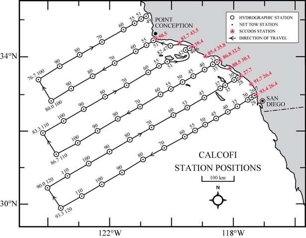
Since 1949, CalCOFI has organized cruises to measure the physical and chemical properties of the California Current System and census populations of organisms from phytoplankton to avifauna. This is the foremost observational oceanography program in the United States.

Currently, 18 to 28 day cruises are conducted quarterly - summer & fall cruises are typically 18 days, winter & spring cruises are longer. Scripps and NOAA provide equally in terms of ship time, personnel, and other cruise-related costs. On each cruise a grid of 75 stations off Southern California is occupied. Winter & spring cruise may occupy stations just north of Pt Conception up to Monterey or San Francisco. At each station a suite of physical and chemical measurements are made to characterize the environment and map the distribution and abundance of phytoplankton, zooplankton, fish eggs and larvae.

Core measurements

• temperature, salinity, oxygen, nutrients
• water masses and currents
• primary production
• phyto- and zooplankton biomass & biodiversity
• meteorological observations
• distribution and abundance of fish eggs & larvae
• marine birds & mammal census; marine mammal acoustic recordings
• fisheries acoustics
   

CalCOFI hydrographic CTD data, particularly the thermodynamic properties, are computed by Seasoft based on EOS-80. Temperatures, typically from the primary temperature sensor, are merged with bottle sample data into station files which produce the hydrographic database and other data products, Hydrographic Reports, figures, IEHs. CTD sensor salinities, and oxygen values may also replace bottle measurements on mistrip or missing samples.

Currently (May 2014) no TEOS-10 calculation for absolute salinities are calculated.

Information from Seasoft v7.23.1 (May 2014)

Algorithms used for calculation of derived parameters in Data Conversion, Derive, Sea Plot, SeaCalc III [EOS-80 (Practical Salinity) tab], and Seasave are identical, except as noted in Derived Parameter Formulas (EOS-80; Practical Salinity), and are based on EOS-80 equations.

Derived Parameter Formulas (EOS-80)

For formulas for the calculation of conductivity, temperature, and pressure, see the calibration sheets for your instrument.
 
Formulas for the computation of salinity, density, potential temperature, specific volume anomaly, and sound velocity were obtained from "Algorithms for computation of fundamental properties of seawater", by N.P. Fofonoff and R.C Millard Jr.; Unesco technical papers in marine science #44, 1983.

• Temperature used for calculating derived variables is IPTS-68, except as noted. Following the recommendation of JPOTS, T68 is assumed to be 1.00024 * T90 (-2 to 35 °C).
• Salinity is PSS-78 (Practical Salinity) (see Application Note 14: 1978 Practical Salinity Scale on our website). By definition, PSS-78 is valid only in the range of 2 to 42 psu. Sea-Bird uses the PSS-78 algorithm in our software, without regard to those limitations on the valid range. Unesco technical papers in marine science 62 "Salinity and density of seawater: Tables for high salinities (42 to 50)" provides a method for calculating salinity in the higher range (http://unesdoc.unesco.org/images/0009/000964/096451mb.pdf).

Read more ...

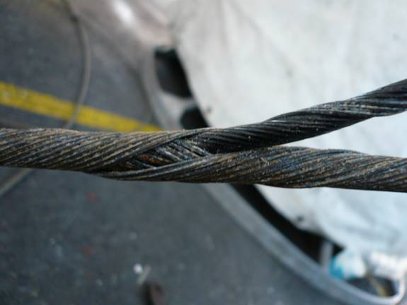
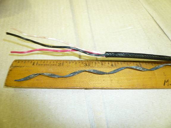
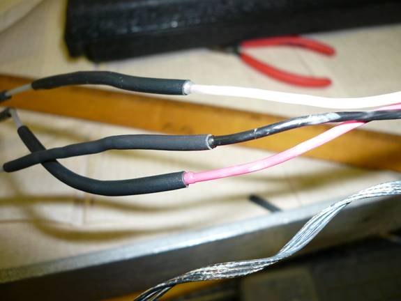
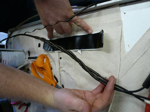
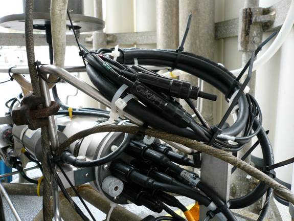
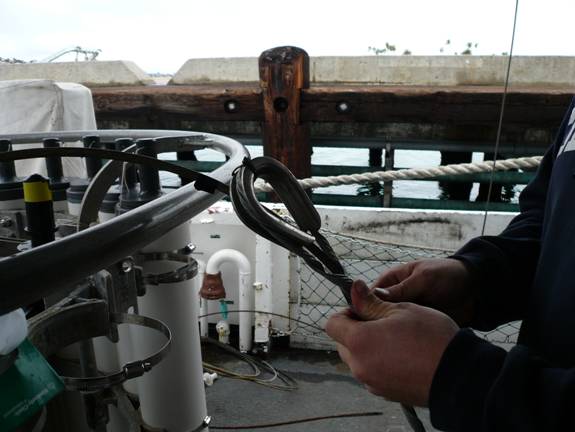
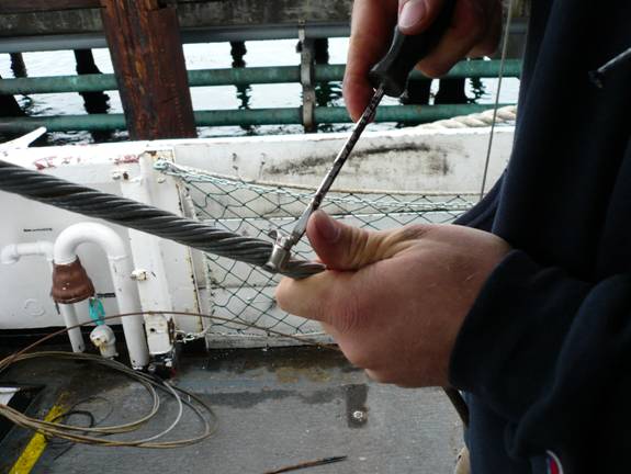
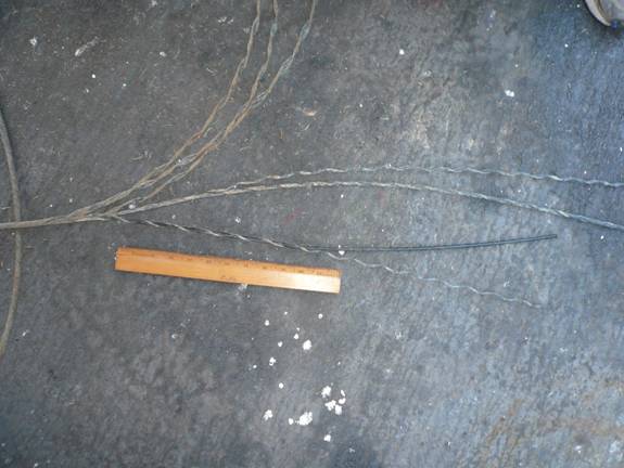
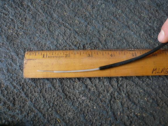
The SIO-CalCOFI method of termination is one of many techniques used to interface a CTD on a conductive wire. Over the years, our method has evolved - this document describes our current technique.
Since many ships have a 3-conductor wire (3 internal wires plus shield), each wire is terminated separately, isolating it from the other wires. If any single conductor fails over the course of the cruise, it can be disconnected from the CTD pigtail without having to re-terminate. Although each of the 3 wires & shield has its own connector, the CTD pigtail can combines the two 'best' conductive wires for the signal, reducing resistance. The remaining conductor is a spare or can be paired with the shield as ground. CalCOFI typically uses only the shield for ground.
On vessels with a single-wire conductive sea-cable, the standard termination (signal=conductive wire; ground=shield) method is used with a Seabird two-pin CTD pigtail. The wire stripping, soldering, and sealing of the termination is done the same way but with only one wire and shield. A standard two-pin Seabird termination pigtail is interfaced with the ship's single conductor wire. Wire shield is used for ground.

Part 1: The termination	(click photos for larger image)
Inspect the conductive wire on the winch drum and cut off any severely rusty or kinked wire. Inspect a few wire strands & bend them back, if brittle, remove additional wire till you find pliable strands. Pull at least 3m (~10ft) of winch wire on deck to allow termination on the wet lab bench top, if available.
Unwrap the outer sheath ~2 m (6ft) length in 2 or 3 groups - keep them organized so rewrapping can be done easily. Unwrap the inner sheath in 2 groups, exposing the conductive wire core then unravel 3 adjacent inner shield strands to keep with the core and use as ground. Trim the plastic core & 3-strands of inner shield to ~50cm (20") from the unwrap point. This will be long enough to terminate & reterminate at least once. Retermination will be required if a solder connection fails or from seawater intrusion.
Rewrap the unravelled shield back into a single, coreless wire, leaving the conductive core & 3 strands exposed. Tape the frayed end of the wire with black electrical tape.
Strip ~8cm (~3") of the black, outer protective core. This is difficult & best done in small, 0.75cm (3/8") increments using coax cable stripper adjusted to cut the outer cover without cutting into the inner conductive wires. Careful when persuading off the black plastic covering you do not damage the conductive wires. Heat may be applied to the plastic covering to soften it, making it more malleable.  Strip ~2.5cm (1") from the ends of the three sea cable conductors, exposing copper wire ends.
After stripping the 3 wire ends, exposing copper, conduct a 9-volt battery test if wire conductive integrity is unknown: Inside the ship, at the CTD sea cable junction box, free the ends of all conductive wires from the wire poles. Attach a 9 volt battery to two conductive wires at the termination end. Note the color & polarity of the wires and, moving back to the junction box, identify the two wires which read ~+9 volts on a multimeter. Record their color & polarity then switch the + battery connection to the other conductor & indentify its corresponding wire at the junction box. The voltage readings will verify you have good conductivity - check for 'cross-talk' by measuring all the wires for voltage leakage. If any wire does not conduct the proper voltage or has a stable voltage reading when it is not connected to the battery, further testing is required to determine if that wire should be excluded from the termination. Repeat, if necessary, until you've color keyed the three conductive wires and shield. Hopefully, the wire colors in the junction box agree with the conductive cable. Connect the conductive wires to the wire poles in the junction box, noting the colors.
Strip ~2.5cm (1") off four single-pin Impulse connectors; the forth one is for the shield. Our CTD pigtail has single-pin male connectors so single-pin female connectors are solder to the sea cable conductors. Use 95% alcohol on a large Kim-wipe to de-grease all the wire surfaces for good adhesion of shrink-tubing, tape, electrical putty & coating. Let dry a few minutes. Be sure to slip on the Impulse connector sleeves before soldering & color code them with tape to match the junction box wires. Use the wire color key from step 10 to coordinate the connector color to the proper junction box wire.
Slip adhesive-lined shrink tubing, trimmed ~1cm (0.5") shorter than the bare wire, up the wire away from the end to be soldered. Solder wires, paying particular attention to not melt shrink tube prematurely. If there are any sharp wire ends protuding from the solder weld, file them smooth. Let the solder weld cool for ~30 seconds then slid the shrink tubing evenly over the weld. Apply heat, starting from the middle and working toward each end, until all air is expelled. Adhesive should seep from both ends of the shrink tubing insuring a good moisture barrier (see photo). For the shield-ground connection, snip off one shield strand then use an emory cloth to remove oxidation & rust from the ends (~4cm) of the remaining two stands. Using a crimp connector, crimp the Impulse connector wire to the two shield strands then fill the crimp with solder. Shrink tubing does not need to be applied to this connection.
Smoothly (no bubbles) apply Scotch-Coat electrical coating to each wire individually. Scotch-coat ~7cm (3") up onto the black core & Impulse connector insulation. Keep all wire separated as they dry 20-30mins. Split 1.9cm (3/4") insulating tape in half with sharp scissors so you have a 0.95cm (3/8") wide piece about 16cm (6") long. Starting ~2.5cm (1") up on the Impulse connector's black insulation, tightly wrap the wire with insulating tape sticky side up. Wrap your way down onto the thinner wire using multiple layers of insulation tape to reinforce and strengthen the thin diameter junction. Stretch and tightly wrap your way up to the black plastic core, stopping where the three conductors come together. Repeat for the two other conductors. For the shield connector, start wrapping 2.5cm up on the Impulse connector's black insulation. Tightly wrap the wire to prevent moisture intrusion under the connector insulation then continue up & over the crimped connector. Apply Scotch-coat to all the individual wires once more and let dry 20-30 minutes. (Optional) Repeat step 18, adding a second layer of insulating tape onto the three main conductive wires. On the third wire, instead of stopping where the three wires meet, continue ~6cm (2.5") up onto the black plastic core with the final wrap Apply Scotch-coat to the four wires and let dry.
Cut a piece of electrical putty tape slightly longer then length of the termination, trim off the four corners and wrap it around all wires like a taco, not however, before twisting all wires together to form a spiral braid. Pinch the putty edges together forming a seamless tube around the termination. Squeeze the putty into the air pockets between the wires - try to eliminate as much trapped air as possible by kneading outward from the middle. Wrap the putty 'tube' with Super 33 electrical tape, starting at the middle and working toward the loose end, wrapping very tightly.  When you reach near the edge, leave 0.5cm of the putty unwrapped, then wrap back to the center normally (tight but not stretching the tape); once back to center, repeat the technique on the other half, wrapping tightly to near the edge then back to middle normally until you've completely double-wrapped the termination. It is important to leave each end open so as the putty compresses, it can seep out the ends.
Apply a final coat of Scotch-coat, sealing the tape surface. Loosely wrap the ground wire to the outside of the termination then tape it in place so all connectors are gathered together.
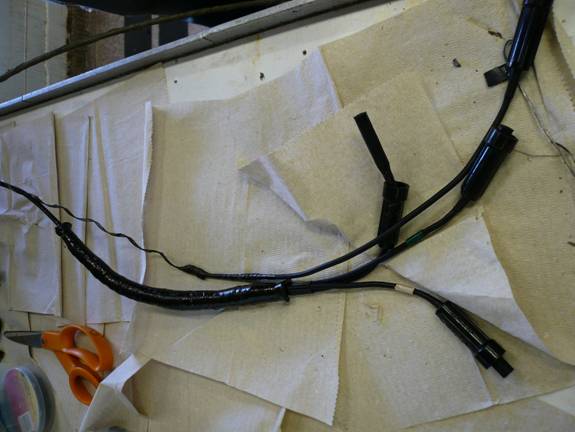Part II: The Sea-cable Connection
Using the cable color key from Part 1 step 10, at the junction box, combine two conductors for signal (usually red & white)  then the third conductor to ground. Using the shield is standard practive but on some ships, it generates electrical noise (spikes). At the CTD, plug in the appropriate connectors to the CTD pigtail - the signal and common (ground) pairs are indicated on the pigtail sleeves (engraved on our pigtail). There are four connectors on the CTD-pigtail but they combine into signal pair & common pair. Turn on the deck unit, if everything is connected properly, the front LED panel should read something other than '0000000000'. If you get zeros, the most common problem is reversal of signal & common. See CTD Diagnostic web page for troubleshooting instructions.
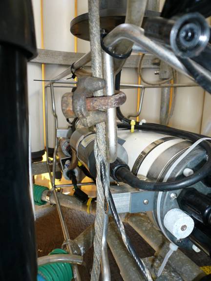
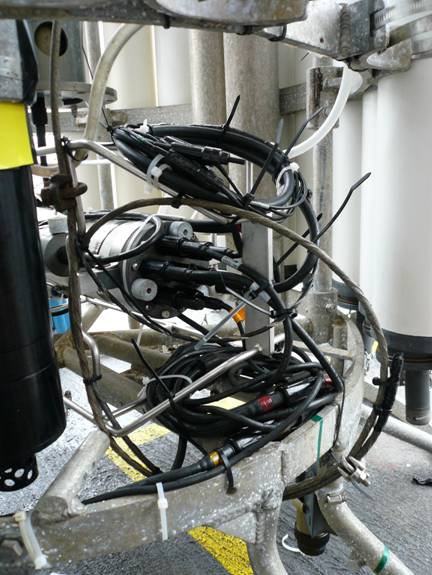
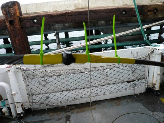
Part III: The Rigging
Disconnect the CTD pigtail from the sea-cable termination. Lacing the wire down through the center of the rosette, loop the termination and sea-cable end once around the rosette frame and along side the CTD cage, paying careful attention to the placement and orientation of the termination.  Adjust the length so the termination & pigtail are easily secured, protected, but accessible when cable harnesses are in place. Use heavy duty cable-ties to secure the sea-cable to itself (loop) and to the frame until cable clamps can be tightened. Place a large cable clamp on the wire and the fish cage (see photo).  This cable clamp immobilizes the conductive wire so when the CTD-rosette is lifted, there is no tension on the termination. Tighten securely but do not over-tighten or you may interrupt the electrical continuity & create a short.
Add two smaller cable clamps on the wire loop about 12cm (5") from the end of the loop and about 40cm (15") from the end of the loop.  Note that the 40cm clamp is not visible in this photo.  This is the main safety for the CTD-rosette should the the guy-wire grip ('Chinese fingers') fail. It is important to be sure the loop does not interfere with the bottle mounting or closure of the bottom lids. SIO-CalCOFI prefers to rig this loop at the end of sea-cable as a safety line should the guy-wire grip slip or fail.
Cable-tie the sea-cable loop to the cage, making sure it does not rub against or interact with CTD sensor cables. Loop the CTD pigtail and sensor cables on the upper or lower cage and secure with multiple cable-ties. It is important the cables not move during the cast especially during rough weather. Double-check all wire & sensor connector sleeves are tight. Make 'shallow' (1000m rated) sensor cables accessible so they can be easily disconnected & dummied when sensors are removed for 3500m casts.
Shackle the sea-cable to rosette frame using a guy-wire grip (guy-cable grip, sometimes called "Chinese Fingers" after the kid's finger trap). Hold the sea-cable up vertically over the rosette center. Allow enough slack so when lifted by the wire grip, there is no tension between the shackle and the cable clamp attached to the CTD cage. This determines the wire grip attachment point up the wire - mark it with black tape. The sea-cable can then be lowered to chest-level for installation. Secure the stainless thimble in the loop of the wire grip with black tape. Begin wrapping the guy-wire grip around the cable. Towards the end, it becomes increasingly difficult to seat the ends of the grip. You may have to use an broad blade screwdriver or tack puller tool to finish the job.
Put a small hose clamp or sturdy cable tie at the top of the guy-wire grip to keep from the ends from unwrapping.
Wrap yellow tape & hi-vis zip ties around wire to help the winch operators' visual determination of optimal 'just below surface'. If the CTD frame shackle has a cotter pin, pass the shackle bolt through the wire grip thimble so that cotter pin is opposite the wire bow. This helps prevent the CTD wire from being pinned under the shackle when slack is removed during deployment. Using 'tuna-cord' or thin nylon line, tie the sea-cable slack out-of-the-way of the bottle lanyards.
Tips & Reminders
The conductive core has a clear tape length index. When unwrapping the core, save the length reading for the ship's cable log. Wire colors can change from the sea-cable to the junction box because the sea-cable conductors are soldered to the junction box wires at the winch's slip rings. This termination can become faulty over the course of the cruise so when troubleshooting signal interruptions, take that into consideration. The longer the length of exposed wire core you leave when unwrapping the shield, the more chances of reterminating without have to unwrap the shield. 50cm (~20") of exposed wire core is enough to reterminate at least once. Cut 2 strands of inner shield approx the same length as the conductive core for ground crimp connection. If you want to use three shield strands, use a larger crimp - we use bare metal crimps that accomodate two shield strands and one Impulse wire. Once the inner connectors are stripped to bare wire, wipe all surfaces of the wire with 95% ethanol to ensure a clean, grease-free connection. Make sure the work space is fairly clean and the work surface is covered with paper towels to catch electrical coating drips. Keep the electrical tapes clean of lint or other debris so wraps are bubble & lint free. If the CTD wire becomes kinked or develop a mechanical weakness in the first several meters (between CTD & winch). It may be possible to continue to use the wire without re-terminating as long as signal continuity is intact. Move the guy-wire grip above the problem area and loop the extra wire along the upper rosette ring. Secure the looped wire with strong cable ties. On ships with side-by-side CTD & Hydro winches: if the CTD conductive wire "jumps the shieve" it may be possible to use the hydro winch to lift the CTD-rosette (or any tethered instrument) and reseat the wire in the shieve. (Restech Bob Wilson 101) Secure the CTD-rosette to the cleats using the taglines to minimize the chances of losing the package if the wire parts. Attach a fresh guy-wire grip to the CTD wire reversed - thimble up, ends down. Switch the hydraulics to the hydro winch. Attach the hydro wire shackle to the guy-wire grip thimble and use the hydro winch to lift the CTD-rosette until there is enough slack to slip the wire back into the shieve. Keep the CTD wire under tension so it stays in place as you carefully pay out wire on the hydro winch. Once the CTD wire is holding the weight of the CTD-rosette, unshackle the hydro wire and remove the wire grip. Return the CTD-rosette to deck and assess any damage to the conductive wire. Reterminate if the integrity of the wire is compromised.

CalCOFI Data Management: Setting Community Standards
(presented as a poster at the 2007 CalCOFI Conference by James Wilkinson, Karen Baker & Richard Charter)

Introduction
CalCOFI represents a partnership of multiple agencies conducting quarterly joint oceanographic cruises. CalCOFI cruise participants work as a cohesive cross-agency unit to accomplish cruise objectives. Ancillary researchers frequently integrate their field measurements and sampling with the long-term core CalCOFI measurements and samples. Once a cruise concludes, however, this cohesive unit disperses; individuals return to their respective agencies and labs to process samples and analyze data. Each group uses legacy lab or agency specific methods and software to generate data products in local formats. These diverse data processing methods, products, and storage formats create challenges for merging final datasets. Development and incorporation of shared data management practices and joint community standards enable data integration.

Establishing Shared Practices
Identifying and establishing common, queriable columns, such as order occupied and event number, and including them in final data products allows heterogeneous datasets to be related. In addition, standardizing data elements such as column headers, date-time specifications, spatial designations such as GPS decimal format are easy to implement with minimal impact on existing data production. Standard, linkable data elements allow ingestion into relational databases, applications, and other analytical tools such as Data Zoo using import templates.

CalCOFI Standardization Strategies:

1. Persistent vocabulary and formats with defined standard data column label
2. Date & position format conventions
   • Date: YYYY/MM/DD HHMMSS.S UTC
   • Position: 32.53455, -117.23433
3. Standard Line Station grid designations example: line 93.3, station 120.0. Traditionally, integer values are used to describe a CalCOFI line.sta, 93.120 for example. But with the integration of SCCOOS stations as part of the regular 75 station pattern, the decimal notation improves line.station distinguishability.
4. Order-occupied numbering for sequential stations
5. Event numbers for distinguishing all station activities that generate data
6. Data distribution in non-proprietary format such as comma-delimited ascii files (.csv) in addition to legacy IEH for data warehouses like NODC who expect & can ingest IEH.
7. Metadata - definitions of measurements & equipment; translation tables for different unit attributes.

Shared Practices Begin in the Field
With quarterly cruises generating a persistent influx of data, the CalCOFI technical team must maintain an established routine to keep pace. Changes in procedure or protocol impact the expediency of the ongoing process. To minimize the impact of new data integration practices, the change process best begins at sea. Careful attention to sta activities & event logs create both a shared index and initiates a dialogue about organizational design.



Figure 1: Typical CalCOFI-SIO Data Flow from Field Collection to Publication


Figure 2: Typical CalCOFI-SWFSC Data Flow from Field Collection to Publication

Developing Data Integration Standards

At sea:

1. Water samples are collected, logged & analysed. Net tows collected, logged, & preserved.
   • Standard 1: all logs use joint standard formats with common station, event number & order occupied indexes.
2. Preliminary data processing and quality control of individual samples types: salinity, nutrients, oxygen, chlorophyll.
   • Standard 2: event logs, sample logs, & analytical output files are available on the network, all include common sample indices.

1. Traditional data processing; merging of individual data types into a combined, local ascii format using in-house software. Preliminary data are merged, quality control protocols are applied. Final compilation and data publication: CalCOFI Data Reports as txt, pdf, and html; contour plots; IEH files (proprietary legacy format), all web accessible.
   • Standard 3: Station & cast information, bottle, and CTD data are merged into a non-proprietary csv with common, queriable elements, standard formats, & labels.
2. Net tow data are processed with the flow meter calibrations and depth of tow, volume of water strained and other variables are calculated and added to the net tow dataset. The bongo tows are then volumed.
   • Standard 4: A plankton volume report is generated with common elements, standard formats and labels.
3. The plankton samples are then sorted removing all fish eggs, larvae and squid paralarvae. The major species (sardine, anchovy, and hake) are identified and sized at the time of sorting. The remaining plankton sample goes to the SIO archives. The unidentified eggs and larvae are identified in the ichthyoplankton identification lab. The fish eggs and larvae are then archived in the NMFS ichthyoplankton archives.
   • Standard 5: An eggs and larvae dataset is produced in a standard format. An annual ichthyoplankton data report is produced in a standard format once all the cruises of the year have been identified.

Cross-Project Data Interfacing

CalCOFI cruises generate multiple data formats such as station data; continuous meteorological, ADCP, & SCIMS (universal format SCS or MET continuous data + event numbers) data; avifauna & marine mammal visual observations and acoustic recordings. Each research group has their own data publishing goals. It must be the goal of all data-producing participants to generate a standard product with common indices for use by the data community. CalCOFI-SIO & CalCOFI-SWFSC are establishing a common vocabulary and standardizing final data formats & practices so hydrographic, zooplankton, and ichthyologic data can be integrated.

Data Interfacing Strategies:

1. Establish a shared data product
2. Consider your final data and what you are able to share with the data community – some data processes take longer.
3. Develop a standard, persistent format so cross-project partners can plan for a consistent data format and design ingestion mechanisms such as import templates.
4. Think collaboratively
5. The Ocean Informatics team is working together to automate the importing of CalCOFI data into DataZoo, a cross-project, web-based, information system.

Acknowledgements
We would like to recognize the added work done by field participants - ship and scientific staff - in helping to plan forward for data integration and by the cross-project community of participants working to create a common information environment. This work is supported by NOAA CalCOFI SIO and SWFSC together with the NSF LTER California Current Ecosystem and the Ocean Informatics team.

This information was presented as a poster at CalCOFI Conference 2007 (image).
Authors: James Wilkinson, Karen Baker from Scripps Institution of Oceanography and Richard Charter from NOAA Southwest Fisheries Science Center
 

Sample Drawing:

1. 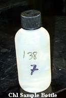Chl samples are drawn on all rosette bottles tripped from ~200m to surface; sampling on a standard 20-bottle cast usually starts at #7 but refer to electronic sample log. For shallow stations, all the bottles may be sampled; noontime prodo casts may have extra bottles to sample; duplicate depths are usually skipped.  Refer to the electronic sample log to verify which bottles to sample or ask the watchleader.

2.  Drawing from the middle valve, add ~20mls, cap loosely, rinse-shake then dump; three rinses.  Double-check the sample bottle number matches the rosette bottle number (often).

3.  Chl samples are volumetric so after rinsing, fill it completely, cap loosely, tap the bottle gently against the rosette frame to dislodge any small bubbles then top-off, cap tightly, invert the bottle – if you see a large bubble, top-off and check again. Squeezing the sides of the bottle can change the sample volume so cup the bottle in your palm during the final fill to minimize this problem.

Read more ...

The graphic below is a reproduction from an article in which researchers at SIO are corroborating these predictions with observations. 

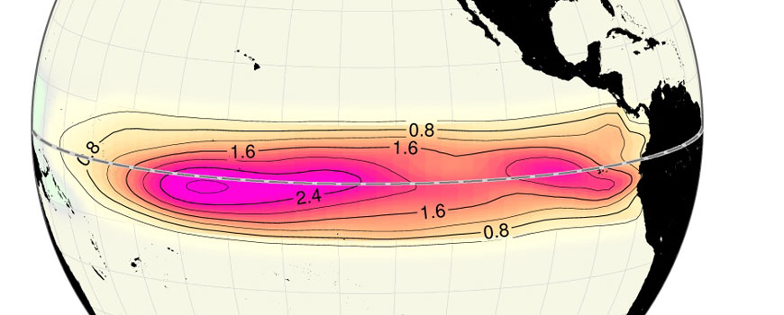
El Niño is an abnormal warming phase in the Pacific Ocean Sea Surface Temperature (SST), while the abnormal cooling is known as La Niña - these shifts are part of the El Niño Southern Oscillation or ENSO.  The current ENSO phase is often quantized by a deviation from normally observed SST using the Oceanic Niño Index or ONI. While El Niño and its counterpart cooling phase La Niña are still being researched, the seasonal effects are becoming well understood with long term data sets.

Using the table below from NOAA's Climate Prediction Center in conjunction with the CalCOFI database - can offer information on how the environment has reacted in response to the different phases and intensities of the ENSO. 

Read more ...

• Retrieve an empty nutrient rack from the lab fridge if needed and record the color key with CESL electronic sample log.
• Wear latex or vinyl gloves; never touch the inside of the cap or tube since residue from your glove can contaminate the sample.  If unavoidable or you drop the lid – rinse several times before capping the sample.
• Nutrients are normally drawn from the middle valve – fill the tube with ~25mls, cap loosely, shake/rinse then dump.  Repeat three times.
• Double check the tube number matches the rosette bottle number.
• Fill the tube completely then flick out several mls so the sample reaches the base of the neck/threads.  Cap tightly.
• Draw one sample per rosette bottle.
• Once all the nutrient samples are drawn:
  • Carefully tip the nutrient rack until you can see the seawater sample through the cap of each tube – if a tube is empty, double-check the sample log and fill if necessary.
  • fill out a sample label (from the sample label clipboard) with the time, your initials, total number of samples
• Wrap the label around tube #1 and carefully re-insert into rack
  • return the filled rack to the nutrient fridge right away.
  • add your initials to the bottom of CESL's sample log’s nutrient column

Common mistakes are empty tubes that shouldn’t be; contaminated samples; and duplicate draws – two sample tubes filled from the same bottle

Seasoft computes PAR using the following equation:

PAR = [multiplier * (10⁹ * 10^{(V-B) / M}) / calibration constant] + offset

Enter the following coefficients in the CTD configuration file:

M = 1.0   (Notes 2 and 3)

B = 0.0   (Notes 2 and 3)

calibration constant = 10⁵ / Cw   (Notes 2 and 4)

multiplier = 1.0 for output units of μEinsteins/m²•sec   (Note 5)

offset = - (10⁴ * Cw * 10^V)   (Note 6)

Notes:

1. In our Seasoft V2 suite of programs, edit the CTD configuration (.con or .xmlcon) file using the Configure Inputs menu in Seasave V7 (real-time data acquisition software) or the Configure menu in SBE Data Processing (data processing software).
2. Sea-Bird provides two calibration sheets for the PAR sensor in the CTD manual:

• Calibration sheet generated by Biospherical, which contains Biospherical’s calibration data.
• Calibration sheet generated by Sea-Bird, which incorporates the Biospherical data and generates M, B, and calibration constant needed for entry in Sea-Bird software (saving the user from doing the math).

3. For all SBE 911plus, 16, 16plus, 16plus-IM, 16plus V2, 16plus-IM V2, 19, 19plus, 19plus V2, 25, and 25plus CTDs, M = 1.0. For SBE 9/11 systems built before 1993 that have differential input amplifiers, M = 2; consult your SBE 9 manual or contact factory for further information. B should always be set to 0.0.
4. Cw is the wet μEinsteins/cm²•sec coefficient from the Biospherical calibration sheet. A typical value is 4.00 x 10 ^-5.
5. The multiplier can be used to calculate irradiance in units other than μEinsteins/m²•sec. See Application Note 11General for multiplier values for other units.
   The multiplier can also be used to scale the data, to compare the shape of data sets taken at disparate light levels. For example, a multiplier of 10 would make a 10 μEinsteins/m²•sec light level plot as 100 μEinsteins/m²•sec.
6. Offset (μEinsteins/m²•sec) = - (10⁴ * Cw * 10^V),  where V is the dark voltage. 
   For typical values (Cw = 4.00 x 10 ^-5 and Dark Voltage = 0.150), offset = -0.5650. 
   The dark voltage may be obtained from:

• Biospherical calibration certificate for your sensor, or
• CTD PAR voltage channel with the sensor covered (dark) — in Seasave V7, display the voltage output of the PAR sensor channel.

Instead of using the dark voltage to calculate the offset, you can also directly obtain the offset using the following method: Enter M, B, and Calibration constant, and set offset = 0.0 in the configuration (.con or .xmlcon) file. In Seasave V7, display the calculated PAR output with the sensor dark; then enter the negative of this reading as the offset in the configuration file.

Mathematical Derivation

1. Using the sensor output in volts (V), Biospherical calculates:
   light (μEinsteins/cm²•sec) = Cw * (10^{Light Signal Voltage} - 10^{Dark Voltage}).
2. Seasoft calculates μEinsteins/m²•sec = [multiplier * 10⁹ * 10^{(V - B) / M}) / Calibration constant] + offset
   where M, B, Calibration constant, and offset are the Seasoft coefficients entered in the CTD configuration file.
3. To determine Calibration constant, let B = 0.0, M = 1.0, multiplier = 1.0. Equating the Biospherical and Seasoft relationships:

10⁴ (cm²/m²) * Cw * (10^{Light Signal Voltage} - 10^{Dark Voltage}) = (10⁹ * 10^V) / Calibration constant + offset

Since offset = - (10⁴ * Cw * 10^{Dark Voltage}), and V = Light Signal Voltage:

Calibration constant = 10⁹ / (10⁴ * Cw) = 10⁵ / Cw

Example: If Wet calibration factor = 4.00 * 10^-5 μEinsteins/cm²•sec, then C = 2,500,000,000 (for entry into configuration file).

Notes:

• See Application Note 11S for integrating a Surface PAR sensor with the SBE 11plus Deck Unit (used with the SBE 9plus CTD).
• See Application Note 47 for integrating a Surface PAR sensor with the SBE 33 or 36 Deck Unit (used with the SBE 16, 16plus, 16plus V2, 19, 19plus, 19plus V2, 25, or 25plus CTD).