CalCOFI CTD data, particularly the thermodynamic properties, are computed by Seasoft based on EOS-80. Temperatures, typically from the primary temperature sensor, are merged with bottle sample data into station files which produce the hydrographic database and other data products, Hydrographic Reports, figures, IEHs. CTD sensor salinities, and oxygen values may also replace bottle measurements on mistrip, interpolated standard levels (in place of calculated interpolations) or missing samples.
Currently (May 2014) no TEOS-10 calculation for absolute salinities are calculated.
Information from Seasoft v7.23.1 (May 2014)
Algorithms used for calculation of derived parameters in Data Conversion, Derive, Sea Plot, SeaCalc III [EOS-80 (Practical Salinity) tab], and Seasave are identical, except as noted in Derived Parameter Formulas (EOS-80; Practical Salinity), and are based on EOS-80 equations.
Derived Parameter Formulas (EOS-80)
For formulas for the calculation of conductivity, temperature, and pressure, see the calibration sheets for your instrument.
Formulas for the computation of salinity, density, potential temperature, specific volume anomaly, and sound velocity were obtained from "Algorithms for computation of fundamental properties of seawater", by N.P. Fofonoff and R.C Millard Jr.; Unesco technical papers in marine science #44, 1983.
- Temperature used for calculating derived variables is IPTS-68, except as noted. Following the recommendation of JPOTS, T68 is assumed to be 1.00024 * T90 (-2 to 35 °C).
- Salinity is PSS-78 (Practical Salinity) (see Application Note 14: 1978 Practical Salinity Scale on Sea-Bird's website). By definition, PSS-78 is valid only in the range of 2 to 42 psu. Sea-Bird uses the PSS-78 algorithm in SBE software, without regard to those limitations on the valid range. Unesco technical papers in marine science 62 "Salinity and density of seawater: Tables for high salinities (42 to 50)" provides a method for calculating salinity in the higher range (http://unesdoc.unesco.org/images/0009/000964/096451mb.pdf). Salinity measurements in the CalCOFI sampling area never been outside the 2 to 42 psu range - typically between 32 - 36 psu.
Derive -- EOS-80 Practical Salinity (excerpt from SBE Data Processing Derive Module)
Derive uses pressure, temperature, and conductivity from the input .cnv file to compute the following oceanographic parameters:
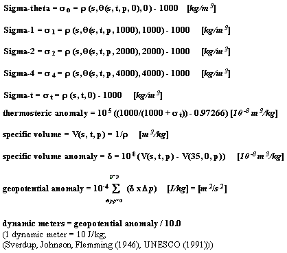
- density (density, sigma-theta, sigma-t, sigma-1, sigma-2, sigma-4)
- thermosteric anomaly
- specific volume
- specific volume anomaly
- geopotential anomaly
- dynamic meters
- depth (salt water, fresh water)
- salinity
- sound velocity (Chen-Millero, DelGrosso, Wilson)
- average sound velocity
- potential temperature (reference pressure = 0.0 decibars)
- potential temperature anomaly
- plume anomaly
- specific conductivity
- derivative variables (descent rate and acceleration) -- if input file has not been averaged into pressure or depth bins
- oxygen (if input file contains pressure, temperature, and either conductivity or salinity, and has not been averaged into pressure or depth bins) -- also requires oxygen current and oxygen temperature (SBE 13 or 23) or oxygen signal (SBE 43)
- corrected irradiance (CPAR)
NOTE
- Calculation of Absolute Salinity and associated parameters (TEOS-10) is available in Derive TEOS-10 and SeaCalc III [TEOS-10 (Absolute Salinity) tab]. Once they are calculated in Derive TEOS-10, they can be plotted in Sea Plot.
Formulas
![]()
(density of seawater with salinity s, temperature t, and pressure p, based on the equation of state for seawater (EOS80))
Density calculation:
Using the following constants –
B0 = 8.24493e-1, B1 = -4.0899e-3, B2 = 7.6438e-5, B3 = -8.2467e-7, B4 = 5.3875e-9, C0 = -5.72466e-3, C1 = 1.0227e-4, C2 = -1.6546e-6, D0 = 4.8314e-4, A0 = 999.842594, A1 = 6.793952e-2, A2 = -9.095290e-3, A3 = 1.001685e-4, A4 = -1.120083e-6, A5 = 6.536332e-9, FQ0 = 54.6746, FQ1 = -0.603459, FQ2 = 1.09987e-2, FQ3 = -6.1670e-5, G0 = 7.944e-2, G1 = 1.6483e-2, G2 = -5.3009e-4, i0 = 2.2838e-3, i1 = -1.0981e-5, i2 = -1.6078e-6, J0 =1.91075e-4, M0 = -9.9348e-7, M1 = 2.0816e-8, M2 = 9.1697e-10, E0 = 19652.21, E1 = 148.4206, E2 = -2.327105, E3 = 1.360477e-2, E4 = -5.155288e-5, H0 = 3.239908, H1 = 1.43713e-3, H2 = 1.16092e-4, H3 = -5.77905e-7, K0 = 8.50935e-5, K1 =-6.12293e-6, K2 = 5.2787e-8
C Computer Code
double Density(double s, double t, double p)
// s = salinity PSU, t = temperature deg C ITPS-68, p = pressure in decibars
{
double t2, t3, t4, t5, s32;
double sigma, k, kw, aw, bw;
double val;
t2 = t*t;
t3 = t*t2;
t4 = t*t3;
t5 = t*t4;
if (s <= 0.0) s = 0.000001;
s32 = pow(s, 1.5);
p /= 10.0; /* convert decibars to bars */
sigma = A0 + A1*t + A2*t2 + A3*t3 + A4*t4 + A5*t5 + (B0 + B1*t + B2*t2 + B3*t3 + B4*t4)*s + (C0 + C1*t + C2*t2)*s32 + D0*s*s;
kw = E0 + E1*t + E2*t2 + E3*t3 + E4*t4;
aw = H0 + H1*t + H2*t2 + H3*t3;
bw = K0 + K1*t + K2*t2;
k = kw + (FQ0 + FQ1*t + FQ2*t2 + FQ3*t3)*s + (G0 + G1*t + G2*t2)*s32 + (aw + (i0 + i1*t + i2*t2)*s + (J0*s32))*p + (bw + (M0 + M1*t + M2*t2)*s)*p*p;
val = 1 - p / k;
if (val) sigma = sigma / val - 1000.0;
return sigma;
}
depth = [m]
(When you select salt water depth as a derived variable, SBE Data Processing prompts you to input the latitude, which is needed to calculate local gravity. SBE Data Processing uses the user-input value, unless latitude is written in the input file header [from a NMEA navigation device]. If latitude is in the input data file header, SBE Data Processing uses the header value, and ignores the user-input latitude.
Note: You can also enter the user-input latitude on the Miscellaneous tab in Data Conversion or Derive, as applicable.)
Depth calculation:
C Computer Code –
// Depth
double Depth(int dtype, double p, double latitude)
// dtype = fresh water or salt water, p = pressure in decibars, latitude in degrees
{
double x, d, gr;
if (dtype == FRESH_WATER) /* fresh water */
d = p * 1.019716;
else { /* salt water */
x = sin(latitude / 57.29578);
x = x * x;
gr = 9.780318 * (1.0 + (5.2788e-3 + 2.36e-5 * x) * x) + 1.092e-6 * p;
d = (((-1.82e-15 * p + 2.279e-10) * p - 2.2512e-5) * p + 9.72659) * p;
if (gr) d /= gr;
}
return(d);
}
seafloor depth = depth + altimeter reading [m]
Practical Salinity = [PSU]
(Salinity is PSS-78, valid from 2 to 42 psu.)
Note: Absolute Salinity (TEOS-10) is available in Sea-Bird's seawater calculator, SeaCalc III. All other SBE Data Processing modules output only Practical Salinity, and all parameters derived from salinity in those modules (density, sound velocity, etc.) are based on Practical Salinity.
Salinity calculation:
Using the following constants
A1 = 2.070e-5, A2 = -6.370e-10, A3 = 3.989e-15, B1 = 3.426e-2, B2 = 4.464e-4, B3 = 4.215e-1, B4 = -3.107e-3, C0 = 6.766097e-1, C1 = 2.00564e-2, C2 = 1.104259e-4, C3 = -6.9698e-7, C4 = 1.0031e-9
C Computer Code –
static double a[6] = { /* constants for salinity calculation */
0.0080, -0.1692, 25.3851, 14.0941, -7.0261, 2.7081
};
static double b[6]={ /* constants for salinity calculation */
0.0005, -0.0056, -0.0066, -0.0375, 0.0636, -0.0144
};
double Salinity(double C, double T, double P) /* compute salinity */
// C = conductivity S/m, T = temperature deg C ITPS-68, P = pressure in decibars
{
double R, RT, RP, temp, sum1, sum2, result, val;
int i;
if (C <= 0.0)
result = 0.0;
else {
C *= 10.0; /* convert Siemens/meter to mmhos/cm */
R = C / 42.914;
val = 1 + B1 * T + B2 * T * T + B3 * R + B4 * R * T;
if (val) RP = 1 + (P * (A1 + P * (A2 + P * A3))) / val;
val = RP * (C0 + (T * (C1 + T * (C2 + T * (C3 + T * C4)))));
if (val) RT = R / val;
if (RT <= 0.0) RT = 0.000001;
sum1 = sum2 = 0.0;
for (i = 0;i < 6;i++) {
temp = pow(RT, (double)i/2.0);
sum1 += a[i] * temp;
sum2 += b[i] * temp;
}
val = 1.0 + 0.0162 * (T - 15.0);
if (val)
result = sum1 + sum2 * (T - 15.0) / val;
else
result = -99.;
}
return result;
}
sound velocity = [m/sec]
(sound velocity can be calculated as Chen-Millero, DelGrosso, or Wilson)
Sound velocity calculation:
C Computer Code –
// Sound Velocity Chen and Millero
double SndVelC(double s, double t, double p0) /* sound velocity Chen and Millero 1977 */
/* JASA,62,1129-1135 */
// s = salinity, t = temperature deg C ITPS-68, p = pressure in decibars
{
double a, a0, a1, a2, a3;
double b, b0, b1;
double c, c0, c1, c2, c3;
double p, sr, d, sv;
p = p0 / 10.0; /* scale pressure to bars */
if (s < 0.0) s = 0.0;
sr = sqrt(s);
d = 1.727e-3 - 7.9836e-6 * p;
b1 = 7.3637e-5 + 1.7945e-7 * t;
b0 = -1.922e-2 - 4.42e-5 * t;
b = b0 + b1 * p;
a3 = (-3.389e-13 * t + 6.649e-12) * t + 1.100e-10;
a2 = ((7.988e-12 * t - 1.6002e-10) * t + 9.1041e-9) * t - 3.9064e-7;
a1 = (((-2.0122e-10 * t + 1.0507e-8) * t - 6.4885e-8) * t - 1.2580e-5) * t + 9.4742e-5;
a0 = (((-3.21e-8 * t + 2.006e-6) * t + 7.164e-5) * t -1.262e-2) * t + 1.389;
a = ((a3 * p + a2) * p + a1) * p + a0;
c3 = (-2.3643e-12 * t + 3.8504e-10) * t - 9.7729e-9;
c2 = (((1.0405e-12 * t -2.5335e-10) * t + 2.5974e-8) * t - 1.7107e-6) * t + 3.1260e-5;
c1 = (((-6.1185e-10 * t + 1.3621e-7) * t - 8.1788e-6) * t + 6.8982e-4) * t + 0.153563;
c0 = ((((3.1464e-9 * t - 1.47800e-6) * t + 3.3420e-4) * t - 5.80852e-2) * t + 5.03711) * t + 1402.388;
c = ((c3 * p + c2) * p + c1) * p + c0;
sv = c + (a + b * sr + d * s) * s;
return sv;
}
// Sound Velocity Delgrosso
double SndVelD(double s, double t, double p) /* Delgrosso JASA, Oct. 1974, Vol 56, No 4 */
// s = salinity, t = temperature deg C ITPS-68, p = pressure in decibars
{
double c000, dct, dcs, dcp, dcstp, sv;
c000 = 1402.392;
p = p / 9.80665; /* convert pressure from decibars to KG / CM**2 */
dct = (0.501109398873e1 - (0.550946843172e-1 - 0.22153596924e-3 * t) * t) * t;
dcs = (0.132952290781e1 + 0.128955756844e-3 * s) * s;
dcp = (0.156059257041e0 + (0.244998688441e-4 - 0.83392332513e-8 * p) * p) * p;
dcstp = -0.127562783426e-1 * t * s + 0.635191613389e-2 * t * p + 0.265484716608e-7 * t * t * p * p - 0.159349479045e-5 * t * p * p + 0.522116437235e-9 * t * p * p * p - 0.438031096213e-6 * t * t * t * p - 0.161674495909e-8 * s * s * p * p + 0.968403156410e-4 * t * t * s + 0.485639620015e-5 * t * s * s * p - 0.340597039004e-3 * t * s * p;
sv = c000 + dct + dcs + dcp + dcstp;
return sv;
}
// sound velocity Wilson
double SndVelW(double s, double t, double p) /* wilson JASA, 1960, 32, 1357 */
// s = salinity, t = temperature deg C ITPS-68, p = pressure in decibars
{
double pr, sd, a, v0, v1, sv;
pr = 0.1019716 * (p + 10.1325);
sd = s - 35.0;
a = (((7.9851e-6 * t - 2.6045e-4) * t - 4.4532e-2) * t + 4.5721) * t + 1449.14;
sv = (7.7711e-7 * t - 1.1244e-2) * t + 1.39799;
v0 = (1.69202e-3 * sd + sv) * sd + a;
a = ((4.5283e-8 * t + 7.4812e-6) * t - 1.8607e-4) * t + 0.16072;
sv = (1.579e-9 * t + 3.158e-8) * t + 7.7016e-5;
v1 = sv * sd + a;
a = (1.8563e-9 * t - 2.5294e-7) * t + 1.0268e-5;
sv = -1.2943e-7 * sd + a;
a = -1.9646e-10 * t + 3.5216e-9;
sv = (((-3.3603e-12 * pr + a) * pr + sv) * pr + v1) * pr + v0;
return sv;
}
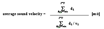
Average sound velocity is the harmonic mean (average) from the surface to the current CTD depth, and is calculated on the downcast only. The first window begins when pressure is greater than a user-input minimum specified pressure and salinity is greater than a user-input minimum specified salinity. Depth is calculated from pressure based on user-input latitude (regardless of whether latitude data from a NMEA navigation device is in the data file).
When you select average sound velocity as a derived variable, SBE Data Processing prompts you to enter the minimum pressure, minimum salinity, and if applicable, pressure window size and time window size.
(Note: You can also enter the parameters on the Miscellaneous tab in Data Conversion or Derive, as applicable.)
-
In Derive, the algorithm is based on the assumption that the data has been bin averaged already. Average sound velocity is computed scan-by-scan:
d i = depth of current scan – depth of previous scan [meters]
v i = sound velocity of this scan (bin) [m/sec] -
In Seasave and Data Conversion, the algorithm also requires user input of a pressure window size and time window size. It then calculates:
d i = depth at end of window – depth at start of window [meters]
v i = (sound velocity at start of window + sound velocity at end of window) / 2 [m/sec]
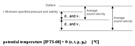
(Potential temperature is the temperature an element of seawater would have if raised adiabatically with no change in salinity to reference pressure pr. Sea-Bird software uses a reference pressure of 0 decibars).
Potential Temperature [IPTS-68] calculation:
C Computer Code
// ATG (used in potential temperature calculation)
double ATG(double s, double t, double p) /* adiabatic temperature gradient deg C per decibar */
/* ref broyden,h. Deep-Sea Res.,20,401-408 */
// s = salinity, t = temperature deg C ITPS-68, p = pressure in decibars
{
double ds;
ds = s - 35.0;
return((((-2.1687e-16 * t + 1.8676e-14) * t - 4.6206e-13) * p + ((2.7759e-12 * t - 1.1351e-10) * ds + ((-5.4481e-14 * t + 8.733e-12) * t - 6.7795e-10) * t + 1.8741e-8)) * p + (-4.2393e-8 * t + 1.8932e-6) * ds + ((6.6228e-10 * t - 6.836e-8) * t + 8.5258e-6) * t + 3.5803e-5);
}
// potential temperature
double PoTemp(double s, double t0, double p0, double pr) /* local potential temperature at pr */
/* using atg procedure for adiabadic lapse rate */
/* Fofonoff,N.,Deep-Sea Res.,24,489-491 */
// s = salinity, t0 = local temperature deg C ITPS-68, p0 = local pressure in decibars, pr = reference pressure in decibars
{
double p, t, h, xk, q, temp;
p = p0;
t = t0;
h = pr - p;
xk = h * ATG(s,t,p);
t += 0.5 * xk;
q = xk;
p += 0.5 * h;
xk = h * ATG(s,t,p);
t += 0.29289322 * (xk-q);
q = 0.58578644 * xk + 0.121320344 * q;
xk = h * ATG(s,t,p);
t += 1.707106781 * (xk-q);
q = 3.414213562 * xk - 4.121320344 * q;
p += 0.5 * h;
xk = h * ATG(s,t,p);
temp = t + (xk - 2.0 * q) / 6.0;
return(temp);
}
![]()
potential temperature anomaly =
potential temperature - a0 - a1 x salinity
or
potential temperature - a0 - a1 x Sigma-theta
(When you select potential temperature anomaly as a derived variable, SBE Data Processing prompts you to enter a0, a1, and the selection of salinity or sigma-theta.
Note: You can also enter the parameters on the Miscellaneous tab in Data Conversion or Derive, as applicable.))
plume anomaly = potential temperature (s, t, p, Reference Pressure) – Theta-B – Theta-Z/Salinity-Z * (Salinity – Salinity-B)
(When you select plume anomaly as a derived variable, SBE Data Processing prompts you to enter Theta-B, Theta-Z/Salinity-Z, Salinity-B, and Reference Pressure.
Note: You can also enter the parameters on the Miscellaneous tab in Data Conversion; plume anomaly is not available as a derived variable in Derive.)
The plume anomaly equation is based on work in hydrothermal vent plumes (Reference: Baker, E.T., Feely, R.A., Mottl, M.J., Sansone, F. T., Wheat, C.G., Resing, J.A., Lupton, J.E., "Hydrothermal plumes along the East Pacific Rise, 8° 40′ to 11° 50′ N: Plume distribution and relationship to the apparent magmatic budget", Earth and Planetary Science Letters 128 (1994) 1-17.). The algorithm used for identifying hydrothermal vent plumes uses potential temperature, gradient conditions in the region, vent salinity, and ambient seawater conditions adjacent to the vent. This function is specific to hydrothermal vent plumes, and more specifically, temperature and potential density anomalies. It is not a generic function for plume tracking (for example, not for wastewater plumes). One anomaly for one region and application does not necessarily apply to another type of anomaly in another region for a different application. The terms are specific to corrections for hydrothermal vent salinity and local hydrographic features near vents. They are likely not relevant to other applications in this exact form.
If looking at wastewater plumes, you need to derive your own anomaly function that is specific to what it is you are looking for and that is defined to differentiate between surrounding waters and the wastewater plume waters.
specific conductivity = (C * 10,000) / (1 + A * [T – 25]) [microS/cm]
(C = conductivity (S/m), T = temperature (° C),
A = thermal coefficient of conductivity for a natural salt solution
[0.019 - 0.020]; Sea-Bird software uses 0.020.)
oxygen [ml/l] = (As applicable, see Application Note 64: SBE 43 Dissolved Oxygen Sensor or Application Note 13-1: SBE 13, 23, 30 Dissolved Oxygen Sensor Calibration & Deployment).
When you select oxygen as a derived variable, there are two correction options available:
-
Tau correction -- The Tau correction ([tau(T,P) * dV/dt] in the SBE 43 or [tau * doc/dt] in the SBE 13 or 23) improves response of the measured signal in regions of large oxygen gradients. However, this term also amplifies residual noise in the signal (especially in deep water), and in some situations this negative consequence overshadows the gains in signal responsiveness.
If the Tau correction is enabled, oxygen computed by Seasave and Data Conversion module are somewhat different from values computed by Derive. Both algorithms compute the derivative of the oxygen signal with respect to time (with a user-input window size for calculating the derivative), using a linear regression to determine the slope. Seasave and Data Conversion use a window looking backward in time, since they share common code and Seasave cannot use future values of oxygen while acquiring data in real time. Derive uses a centered window (equal number of points before and after the scan) to obtain a better estimate of the derivative. Use Seasave and Data Conversion to obtain a quick look at oxygen values; use Derive to obtain the most accurate values. -
Hysteresis correction (SBE 43 only, when using Sea-Bird equation) -- Under extreme pressure, changes can occur in gas permeable Teflon membranes that affect their permeability characteristics. Some of these changes (plasticization and amorphous/crystallinity ratios) have long time constants and depend on the sensor’s time-pressure history. These slow processes result in hysteresis in long, deep casts. The hysteresis correction algorithm (using H1, H2, and H3 coefficients entered for the SBE 43 in the .con or .xmlcon file) operates through the entire data profile and corrects the oxygen voltage values for changes in membrane permeability as pressure varies. At each measurement, the correction to the membrane permeability is calculated based on the current pressure and how long the sensor spent at previous pressures.
Hysteresis responses of membranes on individual SBE 43 sensors are very similar, and in most cases the default hysteresis parameters provide the accuracy specification of 2% of true value. For users requiring higher accuracy (±1 µmol/kg), the parameters can be fine-tuned, if a complete profile (descent and ascent) made preferably to greater than 3000 meters is available. H1, the effect’s amplitude, has a default of -0.033, but can range from -0.02 to -0.05 between sensors. H2, the effect’s non-linear component, has a default of 5000, and is a second-order parameter that does not require tuning between sensors. H3, the effect’s time constant, has a default of 1450 seconds, but can range from 1200 to 2000. Hysteresis can be eliminated by alternately adjusting H1 and H3 in the .con or .xmlcon file during analysis of the complete profile. Once established, these parameters should be stable, and can be used without adjustment on other casts with the same SBE 43.
(When you select oxygen as a derived variable, Data Conversion prompts you to enter the window size (seconds) and asks if you want to apply the Tau correction and the hysteresis correction; Derive prompts you to enter the window size (seconds) and asks if you want to apply the Tau correction.)
Note: You can also enter the window size and enable the correction(s) on the Miscellaneous tab in Data Conversion or Derive, as applicable.
NOTE
Oxygen [ml/l] for the SBE 63 Optical Dissolved Oxygen Sensor is calculated as described in its manual. Tau and hysteresis corrections are not applicable to the SBE 63.
oxygen [mmoles/kg] = 44660 * oxygen [ml/l] / (Sigma-theta + 1000)
Oxygen saturation is the theoretical saturation limit of the water at the local temperature and salinity value, but with local pressure reset to zero (1 atmosphere). This calculation represents what the local parcel of water could have absorbed from the atmosphere when it was last at the surface (p=0) but at the same (T,S) value. Oxygen saturation can be calculated as Garcia and Gordon, or Weiss --
Garcia and Gordon:
Oxsol(T,S) = exp {A0 + A1(Ts) + A2(Ts) 2 + A3(Ts) 3 + A4(Ts) 4 + A5(Ts) 5
+ S * [B0 + B1(Ts) + B2(Ts) 2 + B3(Ts) 3] + C0(S) 2}
where
-
- Oxsol(T,S) = oxygen saturation value (ml/l)
- S = salinity (psu)
- T = water temperature (ITS-90, deg C)
- Ts = ln [(298.15 – T) / (273.15 + T)]
-
A0 = 2.00907 A1 = 3.22014 A2 = 4.0501
A3 = 4.94457 A4 = - 0.256847 A5 = 3.88767 -
B0 = -0.00624523 B1 = -0.00737614
B2 = -0.010341 B3 = -0.00817083 - C0 = -0.000000488682
Weiss:
Oxsat(T,S) = exp {[A1 + A2 * (100/Ta) + A3 * ln(Ta/100) + A4 * ( Ta/100)]
+ S * [B1 + B2 * (Ta/100) + B3 * (Ta/100)2 ]}
where
-
- Oxsat(T,S) = oxygen saturation value (ml/l)
- S = salinity (psu)
- T = water temperature (IPTS-68, deg C)
- Ta = absolute water temperature (T + 273.15)
- A1 = -173.4292 A2 = 249.6339 A3 = 143.3483 A4 = -21.8492
- B1 = -0.033096 B2 = 0.014259 B3 = -0.00170
Notes:
- The oxygen saturation equation based on work from Garcia and Gordon (1992) reduces error in the Weiss (1970) parameterization at cold temperatures.
- As implemented in Sea-Bird software, the Garcia and Gordon equation is valid for -5 < T < 50 and 0 < S < 60. Outside of those ranges, the software returns a value of -99 for Oxsol.
- As implemented in Sea-Bird software, the Weiss equation is valid for -2 < T < 40 and 0 < S < 42. Outside of those ranges, the software returns a value of -99 for Oxsat.
Oxygen, percent saturation is the ratio of calculated oxygen to oxygen saturation, in percent:
(Oxygen / Oxygen saturation) * 100%.
The Oxygen Saturation value used in this calculation is the value that was used in the Oxygen calculation --
- SBE 43 -- if you selected the Sea-Bird equation in the .con or .xmlcon file, the software uses the Garcia and Gordon Oxsol in this ratio; if you selected the Owens-Millard equation in the .con or .xmlcon file, the software uses the Weiss Oxsat in this ratio.
- SBE 13, 23, or 30 -- the software uses the Weiss Oxsat in this ratio.
Nitrogen saturation is the theoretical saturation limit of the water at the local temperature and salinity value, but with local pressure reset to zero (1 atmosphere). This calculation represents what the local parcel of water could have absorbed from the atmosphere when it was last at the surface (p=0) but at the same (T,S) value.
N2Sat(T,S) = exp {[A1 + A2 * (100/Ta) + A3 * ln(Ta/100) + A4 * ( Ta/100)]
+ S * [B1 + B2 * (Ta/100) + B3 * (Ta/100)2 ]}
where
-
- N2Sat(T,S) = nitrogen saturation value (ml/l)
- S = salinity (psu)
- T = water temperature (deg C)
- Ta = absolute water temperature (deg C + 273.15)
- A1 = -172.4965 A2 = 248.4262 A3 = 143.0738 A4 = -21.7120
- B1 = -0.049781 B2 = 0.025018 B3 = -0.0034861
Note: The nitrogen saturation equation is based on work from Weiss (1970).
Descent rate and acceleration are computed by calculating the derivative of the pressure signal with respect to time (with a user-input window size for calculating the derivative), using a linear regression to determine the slope. Values computed by Seasave and Data Conversion are somewhat different from values computed by Derive. Seasave and Data Conversion compute the derivative looking backward in time (with a user-input window size), since they share common code and Seasave cannot use future values of pressure while acquiring data in real time. Derive uses a centered window (equal number of points before and after the scan; user-input window size) to obtain a better estimate of the derivative. Use Seasave and Data Conversion to obtain a quick look at descent rate and acceleration; use Derive to obtain the most accurate values.
(When you select descent rate or acceleration as a derived variable, SBE Data Processing prompts you to enter the window size (seconds).
Note: You can also enter the window size on the Miscellaneous tab in Data Conversion or Derive, as applicable.)
Corrected Irradiance [CPAR] = 100 * ratio multiplier * underwater PAR / surface PAR
(ratio multiplier = scaling factor used for comparing light fields of disparate intensity, input in .con or .xmlcon file entry for surface PAR sensor;
underwater PAR = underwater PAR data;
surface PAR = surface PAR data)
Note: For complete description of ratio multiplier, see Application Note 11S (11plus Deck Unit) or 47 (SBE 33 or 36 Deck Unit).