Please note, the processing methods described use SIO-CalCOFI-developed software (DECODR & BtlVsCTD) to merge and correct Seabird 911+ CTD data with bottle samples. The Seasoft portion of our data processing protocol follow their recommended settings for our 911+ v2 CTD & deck unit.
"Sta.csvs" are bottle data collected at each station cast combined with 1m binavg CTD data from matching bottle depths (~20). Preliminary comparisons & plots of CTD sensor data versus bottle data are generated after each cruise. These comparisons are used to point-check the bottle data and QC the CTD sensor data. Once final bottle data are generated, eliminating fliers & mistrips, a final comparison of 1m binavg CTD to bottle data is performed. This generates final CTD data csv files for each cast that contain 1m binavg Seasoft-processed CTD sensor data, bottle-corrected Seasoft-processed CTD sensor data, and final bottle data.
The CTD temperatures are Seasoft-processed with no additional corrections applied. CTD salinities are corrected using bottle samples from depths >350m, where the profile is near vertical - offset are typically very small (<0.001). CTD SBE43 oxygen data are significantly improved using bottle oxygen samples for calibration; a linear regression is applied to bottle-correct SBE43 O2 profiles. Fluorometer and ISUS-NO3 sensor data require bottle data to generate regressions and convert their voltages to quantitative measurements. Transmissometer & PAR data are collected, processed using Seasoft and not QC'd further. 
Seabird's CTD data processing software suite, Seasoft, is available for free at seabird.com                       JRW 06/2019

CTD Data Processing Quick Guide (rev Jun 2019)

see sections below for more information & settings - these instructions reference SIO-CalCOFI inhouse software which merges CTD & bottle data then applies regression corrections to sensor data based on sensor vs calibration sample plots. CTD data compared to bottle data are 4-second averages prior-to-bottle-closure.

1. Data Conversion... (SBE):  Match CON or XMLCON files accordingly.
    1a. Calculate transmissometer M & B values from deck tests if not done during the cruise, edit/update tranmissometer .xmlcon coefficients to derive beam attenuation coefficients and % light transmission.
2. Window Filter... (SBE):  To smooth profiles & reduce spikes (median filter: 9 for all except cosine 500 for ISUS Voltage, usually setup on V6).
3. Filter... (SBE):  Filter B = 0.15 on Pressure only.
4. Align CTD... (SBE):  Oxygen sensors only (4 seconds).
5. Cell Thermal Mass... (SBE):  Default settings.
6. Derive... (SBE):  Match CON or XMLCON files accordingly.
7. ASCII Out... (SBE):  Select desired variables (see figure below for selection example), check output HDR for errors. DatCNV overwrites the existing .hdr files with new .hdr from embedded information. If the hdr information was keyed-in incorrectly during the cast and the .hdr file was corrected (cast or line.station number, for example) post-cast. The correction is lost when DatCNV generates a new hdr from the .hex file. Hexediting the .hex file, done carefully with a hex editor, will eliminate this problem.
    7a. Sta.csvs updated with .btl data (for 4sec depth value) then 1m .asc data followed by bottle data (salt, O2, chl, nutrients)
8. Step 1... (BTLvsCTD): Individual station BL files and recent preliminary sta.csvs (ieh option still works), unaveraged CTD asc files are required.
9. CSV to .XLS... (Excel):  Open the YYMM_CCTD.CSV generated by BtlVsCTD Step 1 in Excel then save as an XLS file. 
10. Salt... (Excel):  Calculate BTL-CTD offsets (>350m), remove outliers, derive means & statistics.
11. Oxygen... (Excel):  Calculate regressions for both oxygen sensors Sbeox0/1ML/L vs.  BTL_O2.
    11a. Oxygen (Excel):  Calculate regressions for both oxygen sensors Sbeox0/1uM/KG vs.  BTL_O2.
12. Nitrate... (Excel):  Calculate regression for ISUS vs. BTL_NO3.
13. Chlorophyll... (Excel):  Calculate regression for FLSP vs. BTL_CHL.
14. Split... (SBE):  Apply the split to the derived CNV files.  
15. Bin Average... (SBE):  Bin by Depth in 1 meter increments.
16. ASCII Out... (SBE):  Select correct variables.

Generating CTD.csvs for point-checking and plots

17. Step 2... (BTLvsCTD):  ASC- HDR with current sta.csvs (or IEH) and corrected Events file in folder.
18. Plot Profiles... (Matlab):  Plot up cast CSV data with bottles from BTLvsCTD Step 2. 
    18a. Zip & post preliminary CTD+Bottle csvs with metadata files online.
    18b. Copy preliminary CTD+Bottle csvs to dataserver for GTool point-checking.

For Final CTD data, repeat steps 8 - 18 using final data sta.csvs
19. Step 1... (BTLvsCTD): Regenerate comparisons using final sta.csvs (or IEH).
20. Coefficients... (Excel):  Recalculate final regressions and coefficients.
21. Step 2... (BTLvsCTD):  Regenerate final CTD.CSV files.
22. Plot Profiles... (Matlab): Create final up and down cast profiles with bottles.
23. Misc... (BTLvsCTD):  Rename ASC/HDR files, column voltages (optional), and create ZIP files.
24. Database... (Access):  Import files into annual database (usually done by JLW).
25. Data Upload... (WinScp):  Upload files to sio-calcofi.ucsd.edu in correct folders.

Recent Changes

2013 - large data files warehoused on sio-calcofi.ucsd.edu, includes CTD data & underway data
201108 - new sta.csv format replaces 00/20/ieh
5-5-11 Removed Check on Tau Correction during Step One CNV creation. 
5-6-11 No longer plotting downcast without bottles

Recommended SBE Data Processing and BTLvCTD routines for CalCOFI 911 plus Data.

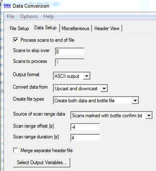
1. Data Conversion... (SBE): Data processor determines whether or not to Match instrument configuration to input file.  If CON file changes during the cruise you will need to match respective CON files to individual stations.  The output CNV files will have header information in them.  It is important to check that each file has the correct line and station information in the header.  Be sure "Create file types" = "Create both data and bottle file". "Source of scan range data" is usually "Scans marked with bottle confirm bit" but if there were non-confirmations, you will have to create a .bsr file for the cast(s). Run Bottle Summary (SBE) on the bottle file to create a .btl file for each cast. This is used to add preliminary 4sec data to the sta.csvs using DECODR's [CTD to Sta.csv] module. Save Data Conversion configuration file (PSA) to cruise folder. 

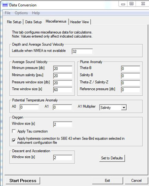
Data Setup / Miscellaneous

  
 

Output variables


 

If .ros files are not generated along with cnv files, rerun Data Conversion to generate ROS files using the BL files as input.  Set ranges to -4 second offset and a 4 second duration. 

Run "SBE Bottle Summary" to convert the ROS file to BTL. Select all of the Averaged Variables and the following Derived variables (as of 2013: add Ox1 & Ox2 in uM/Kg & OxSat1 & 2):

Then using DECODR's [CTD to sta.csv] update the sta.csvs from btl files.

2. Window Filter... (SBE): To be used to remove occasional spikes or dropouts.  Use Median Filter and start with a window of 9 scans.  If spikes last longer than 9 scans open the window wider.  Apply to all variables except ISUS Voltage.  For ISUS apply a 500 scan Cosine Filter to smooth the data.  Save PSA to cruise folder.

3. Filter... (SBE): Use Filter B = 0.15 on Pressure only.  Save PSA to cruise folder.

4. Align CTD... (SBE): The SBE 11plus can be programmed to align data as it is received from the 9plus.  If data is not aligned by the deck unit Align CTD is used.  Regardless of method CNV files are aligned using 0.073 for both Conductivity [S/m] and 4 seconds for both Oxygen Voltage, SBE 43.  Since Fall 2009, both primary & secondary Conductivity [S/m] are corrected by the SBE11 deck unit (v2; note: v1 backup deck unit will only correct the primary conductivity); use Align CTD (4 sec offset) on the Oxygen Voltage(s), SBE43 & Oxygen Raw. Save PSA to cruise folder.

5. Cell Thermal Mass... (SBE): Save PSA to cruise folder.

*Note (optional):  CNV files prior to being Derived and their accompanying CON files can to be archived in a zip file (e.g., 1404CNVpreDerive.zip) so re-deriving later is easier, if necessary. 

6. Derive... (SBE):  Select variables as shown below.  Miscellaneous settings are as shown. Save PSA to cruise folder.

7. ASCII Out... (SBE): For BTLvsCTD Step 1. Compare 4sec CTD processed data to bottle data.  ASCII Out will generate HDR files for each station.  Save as ASCII_Out PSA to cruise folder. Note: if too many variables are selected, Ascii Out will crash. If this happens, unselect the non-essential columns like salinity difference.

Output variables

8. Step 1... (BTLvsCTD): Run Compare 4sec CTD processed data to bottle data. Individual station .BL files and preliminary sta.csvs combine with the unsplit YYMM_###.ASC files.  This routine uses the scan count to average CTD data from each bottle closure to compare with bottle data.  Step 1 outputs individual station and a combined tabulation of CTD and Bottle data, YYMMSSS_avg.CSV and YYMM_CCTD.CSV respectively. This steps can take awhile since the CTD asc files are large.

9. CSV to XLS... (Excel): Open YYMM_CCTD.CSV save as an .XLS file.  Use a previous cruise file as a template if available.

Using the min & max values, exclude any questionable differences – an easy criteria is usually any difference greater than + or – 0.02 (since we are dealing with >350m salts where the salinity profile is nearly vertical).  Just drag outliers to their respective columns.

MATLAB Outlier Calculation - A more rigorous method involves selecting and copying both offset columns into Matlab and generating a box plot.  The box plot function is used to calculate statistical outliers in the data.  Outliers are individually plotted above and below the whisker adjacents.  Select/Copy all data from BTL-Salt00 and BTL-Salt11.  In Matlab create a matrix with the data, create box plots, and mark adjacents values with data tips. Matlab command line statements are as such:

>> salt = [ pastedatahere ];
>> subplot(1,2,1)
>> boxplot(salt(:,1))
>> ylim([-0.01 0.01])
>> title('YYMMSaltOffset00')
>> subplot(1,2,2)
>> boxplot(salt(:,2))
>> ylim([-0.01 0.01])
>> title('YYMMSaltOffset01')

*Note: you may need to adjust ylim boundaries depending on the data

To make Data Tips on the adjacents select the Data Cursor (see below) and Alt-Click on the lines (shown on the right).  It is these Min and Max values that you will use to determine and remove outliers from the data.  Once the figure is complete Save As.. YYMM_SaltOutliers.PNG.

To easily find and exclude outliers sort by offset columns and drag outliers to their respective columns (as shown previously). 

Finally, highlight tabulated data and print selection to PDF (as shown below) saving as YYMM_SaltOffset.pdf.  The mean salinity difference coefficients will be added to the primary & secondary CTD salinities when BTLvCTD is re-run for point-checking.

11. Oxygen... (Excel):  A regression is used to calculate a fit for CTD oxygen data to discrete bottle oxygen data.  Select the two oxygen columns to chart by <Crtl>clicking the two column headers (SbeoxOML/L & Btl_O2 for one; then Sbeox1ML/L & Btl_O2 for the secondary oxygen) then select scatter plot. Move this new chart into its own page and label Ox1 for primary O2 sensor or Ox2 for secondary O2. Repeat for uM/KG, Ox1uM & Ox2uM.  You can also create a separate oxygen worksheet.  Select/Copy/Paste Sbeox0ML/L, Sbeox1ML/L, BTL_Depth, and BTL_O2 columns from the CCTD into the separate oxygen worksheet. In most cases, outliers are not that common nor will they effect the regression calculation.  Four different plots for oxygen will be made each on their own worksheet. Two comparing Sbeox##ML/L to BTL_O2 and two Sbeox##UM/KG to BTL_O2.  All graphs will have Sbeox##ML/L or UM/KG on the x axis and BTL_O2 on the y axis.  All graphs will have linear trend lines (regressions) fit to the data with equations and R² values displayed. Below are examples of how the graphs could look.  These regression coefficients will applied to the primary & secondary CTD oxygen when BTLvsCTD is re-run for point-checking.  Save the graphs with oxygen regression as YYMM_Ox#MLvsOxB.pdf or UMvsOxB.pdf.

12. Nitrate... (Excel):  A regression is used to calculate a fit for ISUS data to discrete bottle nitrate data. Select the ISUS voltage & the Btl_NO3 columns then create a scatter plot. Move the chart to its own page then add the linear regression trendline, including the equation and R². Or you can create a separate nitrate worksheet - select/Copy/Paste Voltage (ISUS), BTL_Depth, and BTL_NO3 columns from the CCTDIEH into the nitrate worksheet. Generate a single worksheet plot, with linear regression, comparing Voltage (ISUS) (x-axis) to BTL_NO3.  Regression equation and R² values need to be displayed. With the exceptions of axes and figure titles and plot marker color, this plot should look similar to that made for oxygen.  These regression coefficients will be applied to ISUS data when BTLvsCTD Step 2 is run for point-checking. Save plot as YYMM_ISUSVvsNO3.pdf.

13. Chlorophyll... (Excel):  A regression is used to calculate a fit for fluorometer data to discrete bottle chlorophyll data.  Select the fluorometer voltage (usually v1) and Btl_Chl columns then create a scatter plot. As with other plots, move the chart to its own worksheet and label Chl. Fit a couple regressions, usually linear or polynomial (sometimes power), to find the best fit. With the trendline, display the equation and R². Or you can create a chlorophyll worksheet.  Select/Copy/Paste fluorometer data (e.g., FLSP or Voltage (fluorometer)), BTL_Depth, and BTL_CHL columns from the main worksheet into the chlorophyll worksheet.  The highly variable nature of fluorometry may require a polynomial or exponential regression to determine best fit; up to a third-order polynomial equation may be applied by Step 2 BTLvsCTD. Outliers may need to be separated from the calculation. The user determines the best method to be applied.  Generate a single worksheet plot, with linear &/or 2nd order polynomial regression, comparing FL Voltage (x-axis) to BTL_CHL.  Regression equation and R² values need to be displayed. With the exceptions of axes and figure titles and plot marker color, this plot should look similar to those made previously.  These regression coefficients will be applied to fluorometer data when BTLvsCTD Step 2 is re-run for point-checking.  Save plot as YYMM_Chla.pdf.

14. Split... (SBE): Apply the split to the derived CNV files.  Output should include up cast and down cast and exclude scans marked bad.  Save PSA to cruise folder. 

15. Bin Average... (SBE): Bin by depth in 1 meter increments.  Include number of scans per bin and exclude scans marked bad.  Skip over zero scans and process up cast and down cast. Save PSA to cruise folder. 

16. ASCII Out... (SBE) ASCII files are necessary for BTLvsCTD Step 2. Correct CTD ASC data then merge w/Btl Data, DB csv out.  Same Data Setup as previously but output variables have changed.  ASCII Out will again generate a HDR file for each station.  Save as ASCII_Out2.PSA to cruise folder.

 Output Variables

17. Step 2... (BTLvsCTD): Run Step 2:Correct CTD ASC data then merge w/Btl Data, DB csv out. Preliminary sta.csvs in the CSV dir or IEH (bigieh or arch.ieh) in the same dir as the CTD ASC files are required.  YYMMEvents.CSV (corrected if available) also needs to be in CTD ASC dir.  It is important that the Event file, if available, is cleaned up and complete. Order occupied, CTD at Depth event number, line and station numbers need to be in order & correct.  Every CTD station requires a "CTD at Depth" event.  If an event was not logged one needs to be added, in doing so the new event number will have an added decimal increment of 0.1 per event.

Step 2: File Selection - Navigate to the ASC folder and select all u*.ASC files.  The d*.ASC files will be automatically processed concurrently.  The leading d or u and trailing box are used to correctly parse the ASC file name to retrieve cruise and station numbers.

Step 2: Sensor Configuration - Using SBE CON or XMLCON files as a guide fill the Voltage Settings boxes.  If different stations had different configurations  (i.e., sensors were moved to different voltage positions on the CTD) process files individually with the correct fields. If a sensor was only removed from the CTD no changes are necessary as the data will be processed as 0.  Fluorescence multiplier and V0 Setting have no effect.

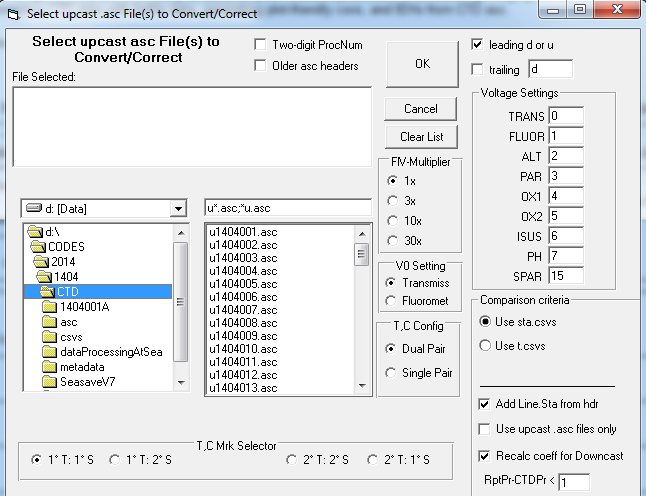
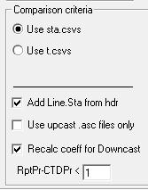Step 2: IEH and Headers - Check the appropriate box for IEH comparison if IEH was selected on the Main Page. If Sta.csvs are used, ignore any ieh setting. Make sure you check Add Line Sta from hdr.  The other two have no effect (legacy remnants).

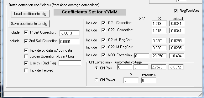
Step 2: Correction Coefficients - Replace the YYMM with the correct cruise designation by highlighting the YYMM in the Coefficients Set dialog. Check the appropriate boxes and enter the necessary coefficients for the required corrections.  If a correction is not being made do not include and enter 0 in the necessary fields.  Also "Include btl data..." and use the -9.990e-29 Bad Flag value to match SBE bad flags.  Save the coefficient CFG to the cruise's CTD directory.

Step 2 will output station CSV files and various combined tabulations of CTD and Bottle data:

18. Plot profiles... (Matlab): Use plotCTDDB600SP.m (or similar) file to plot CTD.CSVs files from BTLvsCTD. Two plots are generated per cast in two formats (png & pdf): 1) downcasts with bottle data, and 2) upcasts with bottle data.

Syntax is:  plotCTDDB600SP ('c:\< data directory>' , ' c:\ ' , 'YYMM' 'u/d' 0/1)

>> plotCTDDB600SP('D:\CODES\2014\1404\CTD\','D:\CODES\2014\1404\CTD\','1404','d',1)

In addition to the input and output file paths, the 'YYMM' is for the Chart Title so edit appropriately; the 'u/d' references up cast data 'u' or 'd' down cast. An unquoted 0 or 1 will toggle the plotting of bottle data on CTD profiles; 1 for bottle data, 0 for no bottle data.  Lately, we've been plotting both up & down cast profiles with bottle data.

Editing plotCTDDB600SP.m may be necessary to accommodate missing data columns and varying cast depths (see variations listed below). Make changes to the file, save it under a different name, then run the new script. This is especially useful when northern lines, which may not have all bottle samples, are best plotted with cruise-averages. This is accomplished by replacing "StaCorr" with "CruiseCorr" in the Matlab script. For deeper casts use:

800m Santa Monica Basin: plotCTDDB800SP('D:\CODES\2014\1404\CTD\','D:\CODES\2014\1404\CTD\','1404','d',1)

3600m Deep Cast: plotCTDDB3600SP('D:\CODES\2014\1404\CTD\','D:\CODES\2014\1404\CTD\','1404','d',1)

Plot Variables: In the m-file there are variables that designate which columns of CSV data to plot.  These can include primary or secondary sensors, and station averages or cruise averages.  You must include depth first then the following CTD then Bottle pairs. For northern lines or stations where bottle sampling is limited (less than 12 bottle samples), cruise-regression corrected CTD data should be plotted.

Variations in Matlab m plot files

For station-regression corrected CTD (corrected using coefficients derived from the station's 20 matching bottle depths):
colHeader = {'Depth','Temp1','BTL_Temp','Salt1_Corr','SaltB',...   
'Ox1_StaCorr','OxB','EstChl_StaCorr','Chl-a','EstNO3_StaCorr','NO3'};

For cruise-regression corrected CTD (corrected using coefficients derived from CTD vs bottle comparisons for all stations):
colHeader = {'Depth','Temp1','BTL_Temp','Salt1_Corr','SaltB',...
'Ox1_CruiseCorr','OxB','EstChl_CruiseCorr','Chl-a','EstNO3_CruiseCorr','NO3'};

Hybrid plots for northern lines where 12 bottle are sampled but no nutrients run, a combination of cruise-corrected nitrate with station-corrected oxygen, chl can be used: 
colHeader = {'Depth','Temp1','BTL_Temp','Salt1_Corr','SaltB',...
'Ox1_StaCorr','OxB','EstChl_StaCorr','Chl-a','EstNO3_CruiseCorr','NO3'};

Axis Labels: Another editable section includes the x axis labels for the above corresponding variables.  Make sure they match up and describe the plotted data pairs accurately.

labels = {'Temperature 0, ITS-90 ','Corrected Salinity 0',...
'Station Calculated Oxygen 0','Station Calculated Chlorophyll A',...
'Station Calculated Nitrate'};

Depth: The last editable field accounts for varying station depths.  Try to group stations together and adjust depth plots accordingly. The below example would plot from surface 0 to 550 meters.

ylim = [-550 0];

*Note... readCTDDBFile.m: The function plotBTLvCTDcsv.m uses this m-file to import the CSV files.  There is one variable that denotes the last column header in the CSV.  Should this value change to addition or reordering of CSV columns it will need to be changed or profiles will fail to plot.  Currently, it is set to: COLHEAD = 'BTL_SIL';

Generating Final CTD.csvs, plots, & metadata

19. Step 1... (BTLvsCTD):After point checking has generated a new set of sta.csvs, final 4-second comparisons need to be calculated.  Run Step 1 as before using final BL, ASC, HDR, and sta.csv (bottle data) files.
This step insures the regression coefficients using final nitrate, oxygen, and chlorophyll data are the best available since point-checking removes errors or mismatches in data and recalculates final values using post-cruise calibration values (fluorometer, for example).

20. Coefficients... (Excel):  Using latest YYMM_CCTD.CSV recalculate regressions and coefficients.

21. Step 2... (BTLvsCTD): Using final coefficients generate final CSV files.  Configure as instructed  previously.

22. Plot Profiles... (Matlab): Create final up cast and down cast profiles with bottles.

23. Misc... (BTLvsCTD); Optional step: Rename ASC & HDR files and column raw CTD voltages. Since sensor may be configured on different voltage channels, this step can insure ambiguous V0, V1,... are relabeled to match the sensor TransV, FluorV....

24. Database... (Access): Import files into annual database. BTLvsCTD generates two compilation files of CTD+bottle data, YYMM_CTDdn.csv & YYMM_CTDup.csv. These will import into the CTD MS Access database fairly straightforward. Open the CTD database and make a backup copy then select External Data, browse to the YYMM_CTDdn.csv file and select Append a copy of the records to the table: YYYY-YYYY_Downcast table. Click OK, then Next, add a check to First Row Contains Field Names, then click Advanced then Specs, select CTD Import Specifications, Open, OK, Next, Finish. If everything is okay, the new data will import into the Downcast table. If not, fix any problems that are tabulated in the Import Error table then rerun. It is ALWAYS a good idea to save a backup copy of the database before updating. Repeat for upcast - please note any corrections needed for the downcast may also be needed for the successful import of the upcast data into the UPCAST (important - remember to pick the Upcast table for the import of upcast data).

25. Data Upload... (FTP/WInSCP or CPanel): upload the CTD zipped files to calcofi.com's download dir. Update the data links on the Available Data page and CTD data pages.

• Collate all files into appropriate subdir then zip
• Metadata subdir
  • YYMM_CTDd.CSV
  • YYMM_CTDu.CSV
  • YYMM_DBcoeff.CSV
  • YYMM_DBcoeff_used.txt
  • YYMM_hdr.CSV
  • YYMM_span.CSV
  • YYMM_xmlcoeff.CSV
  • YYMMEventsFinal.CSV
  • YYMMARCH.IEH (optional)
  • Excel YYMM_CCTD.xls & regression plot pdfs

• Downcast_asc-hdr subdir, contains all .asc & .hdr files relabeled YYMM_LLLLSSSS_###d.asc or .hdr
• Downcast_csv subdir, contains all CTD+Bottle csvs labeled YYMM_LLLLSSSS_###d.csv
• Downcast_plot subdir, contains all YYMM_LLLLSSSS_###d.png or .pdf
• Upcast_asc-hdr subdir, contains all .asc & .hdr files relabeled YYMM_LLLLSSSS_###u.asc or .hdr
• Upcast_csv subdir, contains all CTD+Bottle csvs labeled YYMM_LLLLSSSS_###u.csv
• Upcast_plot subdir, contains all YYMM_LLLLSSSS_###u.png or .pdf

25. Data Backup... : Some archive and working files need to be moved to the CalCOFI file server.  The cruise directory with all original and modified XMLCON, HEX, JPG, etc. need to be placed in a zip file (e.g., 1304archived.zip).  Zip all working files at their various stages that you want to keep in case reprocessing is desired/required.  Zip all PSA files and the YYMM_CCTD.xls & csv files as well. Any special data processing notes, major errors, mislabeling of stations, sensor or termination glitches or changes, should be archived in the metadata zip. Also create a YYMM CTD Data Processing web page with this and any other data processing information worth mentioning.