A station csv (sta.csv) is generated for each CTD cast performed during a cruise. Built from the CTD mrk file, the seawater samples collected from each depth are tabulated. Data columns related to each depth are then populated during sample analysis and data processing. CTD 1-meter bin-averaged data are imported into many columns and used for data quality control, data cross-checks & point-checking. Once populated with final bottle and bottle-corrected CTD data, the sta.csvs are used to generate the CalCOFI data products.
This 2015 revision adds individual datacodes to each nutrient PO4, SIL, NO2, NO3. Previous versions (2014 or older) used either one datacode for PO4, SIL, NO2, & NO3 or individual datacodes merged in the NDC column (P#,S#,T#,O#). NH3 has always had its own datacode. All columns greater than #28 (PO4) in the csv have shifted one to three columns.
Please ignore the DECODR Array column used by our sta.csv data processing program. Its inclusion is for developmental purposes, to facilitate the migration from column-specific programming to dynamic column programming in DECODR.
Bottle Sampling Depths, based on downcast profiles
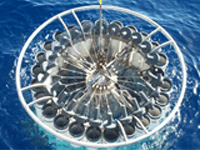 |
The CalCOFI CTD-rosette is equipped with a Sea-Bird Electronic carousel water sampler (SBE 32), a computer-driven, electro-magnetically-released latch system. The 24 ten-liter plastic (PVC) bottles, equipped with epoxy-coated springs & Viton (non-toxic) O-rings, connect to 24 individual triggers by lanyards which keep the bottle ends open. During the downcast, profiles of different sensor measurements vs depth are displayed real-time on a computer screen. Based on the chlorophyll maximum & mixed layer depths, bottles are closed at specific depths to isolate the seawater. The 10 meter bottle spacing shifts up or down (see table below) to resolve steep gradient features such as chlorophyll, oxygen, nitrite maxima and shallow salinity minimum. Salinity, oxygen and nutrients samples are analyzed at-sea for all depths sampled. Chlorophyll-a and phaeopigments samples from the top 200 meters, bottom depth permitting, are also extracted for 24hrs and analyzed at-sea. Most CTD-rosette casts sample 20 depths to a maximum of 515 meters, bottom depth permitting. Occasionally, additional bottle depths or multiple bottles are tripped at the same depth to provide extra water for ancillary projects or primary productivity incubations. Two basin stations, off Santa Monica & Santa Barbara, are sampled beyond 515m to within 10m of bottom. Wire-length permitting, a 3500m deep cast is performed at sta 90.90.
Seabird CTD-Carousel Setup & Deck Unit Diagnostics
 |
 |
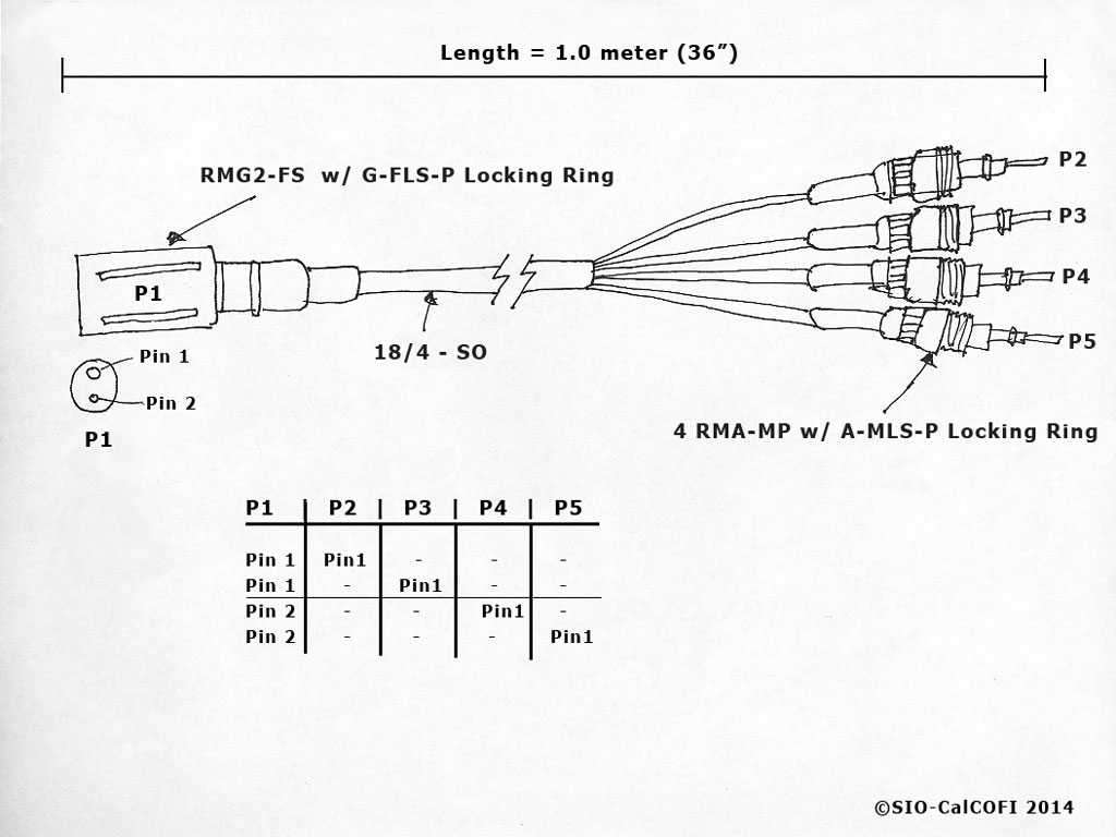
SIO-CalCOFI’s method of terminating the sea cable uses a custom 4-pin pigtail to terminate a multi-strand conductive wire that allows each individual conductor to be used in any combination. Terminating the sea cable using this technique may be viewed in the CalCOFI Handbook: CTD Termination.
Conventional two-pin Seabird pigtail terminations are standard on NOAA vessels and are usually performed by the ET. So interfacing the CTD deck unit only requires the attachment of the sea cable to the deck unit. This is done by connecting a two-conductor wire, such as Seabird part no. 31371 or a coaxial cable equipped with MS3106A connector, from the winch junction box in the CTD lab to the Sea Cable port on the back of the deck unit (see the deck unit section below).
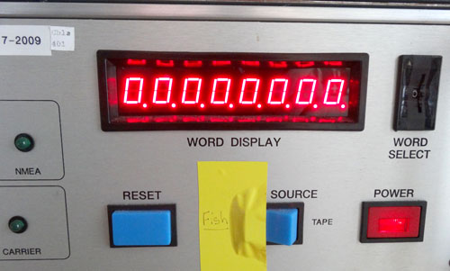
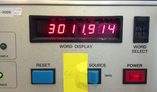
Once the sea cable is connected to the Seabird 9plus and Seabird 11plus deck unit, the deck unit can be powered on. If cabled properly and all electronics are functioning, the numeric LED panel of the deck unit should display non-zero numbers. These values are different for each channel which can be selected by rotating the WORD SELECT dial to the right of the LED panel.
If the LED panel displays “0.0.0.0.0.0.0.0” then the deck unit and CTD “fish” are not handshaking correctly. Turn the deck unit off and wait 60 seconds before touching any exposed wire. Typically, with only two pins, the problem is reversed polarity so switching the wires in the junction box will correct this issue. Please note that powering on the deck unit with reversed polarity may blow the fuse(s). So after switching the wires and before re-powering on the deck unit, check both the 1/2A and 2A fuses on the back of the deck unit & replace if necessary. It is prudent to keep a good supply of these fuses on hand. Power on the deck unit and hopefully, the LED panel has numbers.
Please note in the photos, yellow tape is used to keep the deck unit Signal Source set to Fish. If the switch is toggled to Tape, the deck unit will not communicate with the CTD. The yellow tape prevents the switch from changing from Fish to Tape unintentionally.
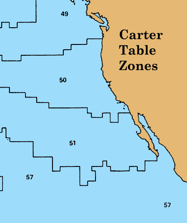 CalCOFI has always corrected bottom depths reported using Carter Tables 50 & 51 for the CalCOFI operations area, California's west coast. An explanation of the need for this correction can be read below and at:
https://www.ngdc.noaa.gov/mgg/fliers/84mgg18.html
"An echo sounding is measurement of the two-way travel time of an acoustic signal between a shipborne transducer and a submerged reflecting surface, usually the ocean bottom. To convert an echo sounding to depth, the travel-time measurement is commonly halved and multiplied by an assumed speed of sound through seawater, either 4,800 ft/sec, 800 fathoms/sec or 1,500 m/sec. The resulting value must be corrected for variations in the speed of sound because of variations in the temperature, salinity, and pressure of sea water. Traditionally, corrections to echo soundings have been interpolated for various areas of the world's oceans from tables published by D.J. Matthews in 1939.* Though the Matthews tables are long outdated, their continued use allowed new depth values to be merged with the large existing data base of depths derived similarly. In 1980, the United Kingdom's Hydrographic Department published a new edition of the correction tables, based on the work of D.J.T. Carter of the United Kingdom's Institute of Oceanographic Sciences.** The Carter tables were adopted in place of Matthews tables by the Twelfth International Hydrographic Conference in Monaco in 1982."
Sample code illustrating CalCOFI stations from Lines 93-77 may be in Carter Table Zone 50 or 51:
If Line in [77, 80, 82, 83, 87, 90, 93] then
Case Line of
77, 80, 82, 83 : Assign(table, 'CARTER50.DAT');
87 : if Sta in [90, 100, 110] then Assign(table, 'CARTER51.DAT')
else Assign(table, 'CARTER50.DAT');
90 : if Sta in [90, 100, 110, 120] then Assign(table, 'CARTER51.DAT')
else Assign(table, 'CARTER50.DAT');
93 : if Sta in [55, 60, 100, 110, 120] then Assign(table, 'CARTER51.DAT')
else Assign(table, 'CARTER50.DAT');
End
DISSOLVED OXYGEN
SUMMARY: The amount of dissolved oxygen in seawater is measured using the Carpenter modification of the Winkler method. Carpenters modification (1965) was designed to increase the accuracy of the original method devised by Winkler in 1889. Using Carpenters modification, the significant loss of iodine is reduced and air oxidation of iodide is minimized. Rather than using the visible color of the iodine-starch complex as an indicator of the titration end-point, we use an automated titrator that measures the absorption of ultraviolet light by the tri-iodide ion, which is centered at a wavelength of 350 nm.
1. Principle
Manganous chloride solution is added to a known quantity of seawater and is immediately followed by the addition of sodium hydroxide iodide solution. Manganous hydroxide is oxidized by the dissolved oxygen in the seawater sample and precipitates forming hydrated tetravalent oxides of manganese.
Mn+2 + 2OH- ----------------------------------------------> Mn(OH)2 (solid)
2Mn(OH)2 + O2 --------------------------------------------> 2MnO(OH)2 (solid)
Upon acidification of the sample, the manganese hydroxides dissolve and the tetravalent manganese in MnO(OH)2 acts as an oxidizing agent, setting free iodine from the iodide ions.
Mn(OH)2 + 2H+ -------------------------------------------> Mn+2 + 2H2O
MnO(OH)2 +4H+ +2I ------------------------------------> Mn+2 +I2 +3H2O
The liberated iodine, equivalent to the dissolved oxygen present in the sample, is then titrated with a standardized sodium thiosulfate solution and the dissolved oxygen present in the sample is calculated. The reaction is as follows:
I2 + 2S2O3 --------------------------------------------------> 2I + S4O6
2. Reagent Preparation
2.1. The manganous chloride solution (3M) is prepared by dissolving 600g of reagent grade manganous chloride tetrahydrate, MnCl2•4H20, in Milli-Q water to a final volume of 1 liter. This solution is then filtered using 47mm glass fiber filters (Whatman GF/F).
2.2 The sodium hydroxide (8M)-sodium iodide (4M) solution is prepared by first dissolving 600g sodium iodide (NaI) in approximately 600ml Milli-Q water. After the NaI is dissolved, 320g of NaOH is added slowly (caution-the solution will get hot) and the volume is adjusted to 1 liter with Milli-Q. The solution is then filtered through a GF/F.
2.3. Sulfuric acid solution (10N) is prepared by slowly adding 280ml of reagent grade concentrated sulfuric acid, H2SO4, to 770ml of Milli-Q water. This should be prepared with caution as is gets very hot.
2.4. The sodium thiosulfate solution (0.2N) is prepared by dissolving 50g sodium thiosulfate pentahydrate (Na2S2O3.5H20) and 0.1g anhydrous sodium carbonate (Na2CO3) in Milli-Q water to a final volume of 1 liter. This solution is prepared approximately 2 weeks before use and stored in an amber glass bottles.
2.5. The potassium iodate standard (0.0100N) is prepared by first drying potassium iodate(KIO3) in a drying oven for approximately one hour. Once the KIO3 is dried, carefully measure out 0.3567g, using a 5-place balance, and dissolve in Milli-Q water to a final volume of 1 liter.
3. Sample Drawing
3.1. Oxygen samples are always drawn first from the Niskin bottles and should be drawn as soon as possible to avoid contamination from atmospheric oxygen. Approximately 6 inches of Tygon tubing connected to a temperature probe via a y-connector is slipped onto the discharge valve of the Niskin.
3.2. A calibrated volumetric flask is rinsed three times, then with the seawater still flowing, the end of the tygon tubing is placed into the flask nearing the bottom. The sample is then overflowed with twice the sample volume while making sure that there are no bubbles in the tubing during the overflow process. The tubing is then carefully removed from the sample flask to prevent the influx of bubbles.
3.3. Immediately after drawing the sample, 1 ml of manganous chloride solution is added into the flask. This is followed by the addition of 1ml of sodium hydroxide-sodium iodide solution to the sample. Both dispensers should be purged to remove air bubbles prior to the addition of these reagents.
3.4. The stopper is then carefully placed in the bottle to avoid the trapping of air and the temperature of the seawater at the time of sample draw is recorded.
3.5. After all samples are drawn, they are shaken vigorously to disperse the precipitate uniformly through the flask. This process is repeated again after the precipitate has settled to the bottom of the flask, or after at least ten minutes.
4. Standardization of thiosulfate
4.1. Proper care in the setup of the auto-titrator is required before running blanks, standards and samples. The UV lamp is turned on at least 30 minutes prior to the run and should have a stable voltage of 2.4-2.5 volts for the run. The dosimat tubing is carefully purged so that the lines are completely free of air bubbles, and the water bath inside the auto-titrator is clean and filled with Milli-Q water prior to analysis. Make sure, prior to your first run, any thiosulfide solution is rinsed off the tip of the line with Milli-Q after purging.
4.2. Using a Metrohm 655 Dosimat, dispense 10 ml of the standard potassium iodate solution into a clean oxygen flask. Add a stir bar and rinse down the sides with a small amount of Milli-Q water. Add 1 ml of the 10N sulfuric acid solution and swirl to ensure the solution is well mixed before adding the pickling reagents.
4.3. Add 1 ml sodium hydroxide-sodium iodide solution to the acidified flask and swirl gently. Then add 1ml of Manganous chloride solution, swirl gently, and fill the solution to the neck of the flask with Milli-Q water.
4.4. The UV detector on the auto-titrator measures the transmission of ultra-violet light through the standard (as well as seawater sample and blank) as a Metrohm 665 Dosimat dispenses thiosulfate at increasingly slower rates. The endpoint is reached when no further change in absorption is detected by the detector. At this point all of the iodine has been consumed.
5. Blank determination
5.1. Using the Metrohm 655 Dosimat, dispense 1 ml of the standard Potassium Iodate solution into a clean oxygen flask. Add a stir bar and rinse down the sides with a small amount of Milli-Q water. Add 1 ml of the 10N sulfuric acid solution and swirl to ensure the solution is well mixed before adding the pickling reagents.
5.2. Add 1 ml sodium hydroxide-sodium iodide solution to the acicified flask and swirl gently. Then add 1ml of Manganous chloride solution, swirl gently, and fill the solution to the neck of the flask with Milli-Q water. The solution is then titrated to the end-point as described in section 4.3 above.
5.3. A second 1 ml aliquot is added to the same solution which is then titrated to a second end-point. The difference between the first and second titration is used as the reagent blank.
6. Sample analysis
6.1. Samples are analyzed after all of the precipitate settles to the bottom of the flask, after the second shake. The top of the flask is wiped with a kimwipe to remove moisture containing excess reagent around the stopper and then the stopper is carefully removed.
6.2. 1ml of 10N sulfuric acid is added to the sample and a stir bar is placed inside the flask. The flask is then secured inside the clean water bath. The tip of the thiosulfate dispenser is placed inside the sample flask and the automated titration can begin with the use of an auto-titrator program.
7. Certified Standard Comparison
7.1 Presented here are the results of a comparison of several certified standards with a CalCOFI prepared standard (weighed and diluted up to set normality in 1 liter volumetric)standard. Three certified iodate solutions, (Table 1) were tested using the same 0.2N thiosulphate solution. Iodate concentrations are back calculated from defined thiosulphate concentrations for comparison purposes. It is noteworthy that the Acculute and Fisher solutions had to be diluted before use. The same volumetric was used for all dilutions, the same Dosimat and piston was used for all titrations, extensive rinsing between uses. Titration n=9 as dictated by the maximum number of samples that could be acquired from the 100ml portion for the OSIL standard. CalCOFI values are a result of cruise and shore based titrations to demonstrate an integrated real use sampling. Differences between all standards represent less than +/- 0.5 percent of the signal.
|
Average[KIO3] mM |
STDEV mM |
% Diff from CC mM |
|||
|
CalCOFI iodate 12/16/2012 used on 1301 |
|||||
|
10.015722 |
0.009609 |
n.a. |
|||
|
OSIL iodate oxygen standard |
|||||
|
9.972671 |
0.013310 |
99.57 |
|||
|
Acculute iodate Lot 00702 |
|||||
|
10.049259 |
0.007684 |
100.33 |
|||
|
Fisher iodate Lot 125009 |
|||||
|
10.044804 |
0.007650 |
100.29 |
|||
7.2 These results are consistent with previously published methods comparison for precision of oxygen measurements1 (WOCE Report 73/91) and previous replicate analysis to verify precision with auto-titration methods2. Although the Ocean Data Facility (ODF) performed the 1991 comparisons for Scripps and was different than CalCOFI, the Winkler techniques used then and now are the same. Presently, CalCOFI methods employ a UV end point auto-titrator made by ODF that produces a precision of 0.005-.01 ml/L. The difference between high and low samples in replicate analysis equals ~0.5% with a standard deviation typically under 0.010 ml/L. See references:
8. Calculation and Expression of Results
8.1. The auto-titrator uses a UV detector that detects changes in voltage as thiosulfate is added to the sample. The volume of thiosulfate added is recorded at an endpoint once there is no change in voltage. The end point is determined by a least squares fit using a group of data points just prior to the end point, where the slope of the titration curve is steep, and a group of data points just after the endpoint, where the slope of the curve is close to zero. The intersection of the two lines is taken as the endpoint.
8.2. The calculation of dissolved oxygen follows the same principle oulined by Carpenter (1965). Our results are expressed in mL/L.
O2(ml/L)= --------------------------- - ---------
Where:
R= Sample titration (mL)
Rblk = Blank value (mL)
VIO3 = Volume of KIO3 standard (mL)
NIO3 - Normality of KIO3 standard
E = 5,598 mL O2/equivalent
Rstd = Volume used to titrate standard
Vb - Volume of sample bottle
Vreg = Volume of reagents
DOreg = Oxygen added in reagents
9. Equipment/Supplies
- Volumetrically calibrated 100ml Glass Erlenmeyer flasks with paired ground glass stoppers
- 3 - 1ml Brinkman reagent dispensers
- Tygon tubing
- Fisher Scientific UV Longwave Pencil Lamp, 365 nm and power supply, 115 VAC
- 2 Metrohm Dosimat 665 Automatic Burets
- 10ml Metrohm Dosimat Exchange unit
- 1ml Metrohm Dosimat Exchange unit
- Metrohm Dosimat Keypad
- Spare 1ml and 10ml dispensor pistons for the Metrohm Dosimat Exchange units
- Scripps/STS Auto-titrator Unit and Software
- PC Computer
- Waterproof sampling thermometer
- Concentrated Sulfuric Acid, H2SO4, ACS Grade
- Manganous Chloride Tetrahydrate, MnCl2•4H20, ACS Grade
- Sodium Hydroxide, NaOH, ACS Grade
- Sodium Thiosulfate, Na2S2O3•5H20, ACS Grade
- Potassium Iodate, Dry high purity KIO3, Alfa Aesar
- Granular Sodium Iodide, EMD Chemicals via VWR
- Magnetic Stir Bars
10. References
- Anderson, G. C., compiler, 1971. "Oxygen Analysis," Marine Technician's Handbook, SIO Ref. No. 71-8, Sea Grant Pub. No. 9.
- Carpenter, J. H., 1965. The Chesapeake Bay Institute technique for the Winkler dissolved oxygen method. Limnol. Oceanogr., 10: 141-143.
- Culberson, C. H. 1991. Dissolved oxygen. WHP Operations and Methods -- July 1991.
- Parsons, T. R., Y. Maita, C. M. Lalli, 1984. A Manual of Chemical and Biological Methods for Seawater Analysis. Pergamon Press Ltd., 3-28.
CalCOFI deploys a Seabird 911+ CTD with 24-place Seabird carousel mounted inside a 24-10L bottle, epoxy-coated rosette frame. Bottle sampling is based on the historical "bottles-hung-on-wire" sampling method utilized by CalCOFI oceangraphers from 1949-1993. Twenty Niskin (5L), Nansen (1.25L), or Wally (2.5L) bottles with messengers were attached to a winch wire and suspended vertically in (typically) 500m of ocean depth. The spring-loaded bottles go into the ocean open so seawater can easily flush through them. Once all 20 bottles were deployed and after a 10+ minute soak for the reversing thermometers to equilibrate. A messenger - 1-2lb metal weight that can clamp & slide freely on the wire - was clamped to the wire and released, dropping onto the first bottle submerged at surface. When closed, the bottles trap seawater from a particular depth with a water-tight seal. This is important since the characteristics of seawater such as salinity and oxygen change with depth. It is critical to the integrity of the measurement that the bottles do not leak and become contaminated by seawater from different depths.
- Nansen bottles: the top end of the Nansen bottle would release from the wire, inverting the bottle, releasing its messenger. The inversion of the thermometers would "break" the mercury in the reversing thermometers, locking in the temperature readings. When inverted, the open bottle ends closed, trapping seawater from that depth for later analyses. Three thermometers - two protected, one unprotected were used on bottles 200m and deeper to derive corrected bottle depth; two thermometers were mounted on bottle shallower than 200m. The released messenger would slide down the wire to trip the next bottle - this would continue until all 20 bottles had closed. Calculating actual bottle depth by comparing protected and unprotected reversing thermometer readings would correct for any inaccuracy due to wire angle or winch-error. In use by CalCOFI 1949 - 1966, and occasionally after until CTD-Rosette implimentation in 1993.
- Niskin bottles: the messenger would strike a plunger, releasing a rotating thermometer rack that would spin 180°, "breaking" the mercury to lock-in the temperature readings of the reversing thermometers. An internal spring would close the o-ringed end caps trapping seawater. CalCOFI Niskins were metal-free & latex-free to allow 14C primary productivity incubation experiments to be conducted with the seawater collected. Epoxy-coated springs and viton o-rings were used to reduce latex toxicity and iron fertilization. After the 1st bottle tripped, the messenger would travel down the wire to the next bottle and so on. The person dropping the messenger would often hold the wire to feel the vibration up the wire of the bottles closing. Eight minutes would elapse for all the bottles to close before the bottle array would be recovered. In use by CalCOFI 1966-1993.
- "Wally" bottles were 2.5L PVC/ABS bottles designed by CalCOFI techs George Anderson & Walt Bryant, similar to Niskins but easier to deploy. They used a single broad wire book-clamp and collected smaller water volumes so were easier-quicker to attach and remove from the wire. They also used epoxy-coated springs and Viton o-rings. During their use, 2.5L of seawater was plenty of volume for the at-sea analyses: salts, nutrients, chlorophylls, oxygens. Like Niskin bottles, after the surface bottle tripped, the messenger would travel down the wire striking the next bottle plunger, closing the bottle, and releasing the next messenger. In use by CalCOFI 1988-1993.
- CTD-rosette: 10L PVC/ABS plastic bottles are equiped with epoxy-spring loaded with Viton o-rings on all surfaces that contact the seawater samples. Unlike a series of bottles clamped to a winch wire, the CTD-rosette is tethered and deployed on a electrically-conductive winch wire. 24-10L bottles encircle the CTD electronics and are rigged open using lanyards attached to the central carousel hub. The CTD sensors display real-time seawater measurements to a computer screen on the ship for the operator & other scientists to see. Based on the downcast profiles of chlorophyll-a and mixed layer depth, as the CTD-rosette is raised, bottles are closed electronically at specific depths by the operator. Reversing thermometers have been replaced by dual CTD temperature sensors. Bottles still trap seawater from specific depths in leak-proof bottles for analyses on-board the ship. In use by CalCOFI 1993-present.
| Line | Sta (if calculated) | Latitude N | Longitude W |
| 93.3, 93 | 26.2 | 32.978982 | -117.272386 |
| 90.0 | 27.6 | 33.497430 | -117.741800 |
| 86.7, 87 | 32.1 | 33.917500 | -118.430800 |
| 83.3, 83 | 39.1 | 34.273350 | -119.308200 |
| 80.0 | 50.3 | 34.474500 | -120.476500 |
| 76.7, 77 | 47.23 | 35.148000 | -120.653000 |
| 73.3, 73 | 49.6 | 35.653333 | -121.221667 |
| 70.0 | 50.9 | 36.196667 | -121.723333 |
| 66.7, 67 | 46.9 | 36.903333 | -121.845000 |
| 63.3, 63 | 49.3 | 37.398333 | -122.425000 |
| 60.0 | 49.0 | 37.988333 | -122.815000 |
Basic Source Code (translated from F77 Fortran)
Public Static Sub OLDDS(LAT1!, Lon1!, D!, Liine$)
'C
'C -- ROUTINE TO RETURN DISTANCE IN NAUTICAL MILES GIVEN TWO POSITIONS
'C IN DECIMAL DEGREES. USES A METHOD THAT WILL MATCH THE RESULTS
'C PRODUCED IN THE OLD VERTICAL SECTION PROGRAM.
'C
'C -> LAT0 -- LATITUDE OF FIRST POINT. (DECIMAL DEGREES. SOUTH NEGATIVE.)
'C -> LON0 -- LONGITUDE OF FIRST POINT. (WEST NEGATIVE)
'C -> LAT1 -- LAT. OF SECOND POINT.
'C -> LON1 -- LONG. OF SECOND POINT.
'C <- D -- DISTANCE (NAUTICAL MILES) BETWEEN POINTS.
'C
Dim COSD#
' Real LAT1, LON1, LAT2, LON2, D
' Real L, DLO, COSD, PI, F, A
PI# = 3.141592654
F# = PI# / 180
'C
' INTRINSIC COS,ABS,SQRT
'C
'COSD#(A#) = Cos(A# * F#)
If frmSelData.txtDataIn(6) = "" Then
LineIn! = (Val(Liine$))
Else
LineIn! = Val(frmSelData.txtDataIn(6))
End If
D! = 0
Dist2Orig$ = ""
190
Select Case CInt(LineIn!)
Case 93, 94 ', 93.3
Lat0! = 32.969 '93.3 26.2 Google projection 2010; old value 32.95298 from Ralf & Nav Program
Lon0! = -117.2696 'Google projection 2010; old value -117.2664
Case 90, 91
Lat0! = 33.49743 '90.0 27.6 Google checked 2010 '4969634422
Lon0! = -117.7418 '745017037
Case 87, 86 ', 86.7
Lat0! = 33.9175 '86.7 32.1 Google projection 2010; old .89568 '918195424
Lon0! = -118.4308 'Google projection 2010; old .419 '431669307
Case 83, 84 ', 83.3
Lat0! = 34.27335 '83.3 39.1 Google checked 2010 '2739356345
Lon0! = -119.3082 '310048755
Case 80, 79
Lat0! = 34.4745 '80.0 50.3 Google projection 2010; old .4631 '4823190269
Lon0! = -120.4765 'Google projection 2010; old .4739 '485679527
Case 77, 76 ', 76.7
Lat0! = 35.148 '76.7 47.23 Google checked 2010 '1446809515
Lon0! = -120.653 '650653673
Case 73 ', 73.3
Lat0! = 35.6533333333
Lon0! = -121.221666667
Case 70
Lat0! = 36.1966666667
Lon0! = -121.723333333
Case 67 ', 66.7
Lat0! = 36.9033333333
Lon0! = -121.845
Case 63
Lat0! = 37.3983333333
Lon0! = -122.425
Case 60 ', 57.8, 57.9
Lat0! = 37.9883333333
Lon0! = -122.815
Case Else
Select Case LineIn!
Case 91.7, 91.6, 91.8, 92
Lat0! = 33.25773 'from Ralf & Nav Program
Lon0! = -117.4385
Case 88.5, 88.6, 88.4, 88
Lat0! = 33.69985 'from Ralf & Nav Program
Lon0! = -118.0522
Case 85.4, 85.5, 85.6
Lat0! = 34.01588 'from Ralf & Nav Program
Lon0! = -118.8243
Case 82, 81.9, 82.1
Lat0! = 34.435 'from Ralf & Nav Program
Lon0! = -119.955
Case 81.7, 81.8, 81
Lat0! = 34.4174 'from Ralf & Nav Program
Lon0! = -119.8033
Case 78.5, 78.4, 78.6
Lat0! = 34.77699 'from Ralf & Nav Program
Lon0! = -120.6302
Case Else
If LineIn! <> Val(Liine$) And LineIn! <> Val(StndL$) Then
LineIn! = Val(StndL$)
GoTo 190
Else
Exit Sub
End If
End Select
End Select
'C
Lon0! = Lon0! * -1
L! = Abs(LAT1! - Lat0!)
DLO! = Abs(Lon1! - Lon0!)
If (DLO! > 180) Then DLO! = 360 - DLO!
'C
L! = L! * 60
DLO! = DLO! * 60
DLO! = DLO! * Cos(F# * ((Lat0! + LAT1!) / 2))
D! = (Sqr(L! * L! + DLO! * DLO!)) * -1
Dist2Orig$ = Format(D!, "#0.00")
If D! = 0 Then Dist2Orig$ = ""
End Sub
Chlorophyll Determination
SUMMARY: Chlorophyll a is extracted in an acetone solution. Chlorophyll and phaeopigments are then measured fluorometrically using an acidification technique.
1. Principle
Seawater samples of a known volume are filtered (< 10 psi) onto GF/F filters. These filters are then placed into 10ml screw-top culture tubes containing 8.0ml of 90% acetone. After a period of 24 to 48 hours, the fluorescence of the samples is read on a fluorometer. Then samples are acidified to degrade the chlorophyll to phaeopigments (i.e. phaeophytin) and a second reading is taken. The readings prior to and after acidification are then used to calculate concentrations of both chlorophyll a and 'phaeopigment'. The method used today is based on those developed by Yentsch and Menzel (1963), Holm-Hansen et al. (1965) and Lorenzen (1967). Note that concentrations of 'phaeopigments' are not a good measure of Chl a degradation products present in the sample since Chl b present in the sample will be measured as 'phaeopigments'.
2. Sample Drawing
|
2.1. |
Chlorophyll bottles should be rinsed three times with sample prior to filling. The bottles are calibrated for volume, so the sample drawer must insure that air bubbles are not clinging to the sides of the bottle and it is filled completely. The sensitivity of the fluorometric method allows for sample bottles of ~50 to 250 ml. |
3. Sample Filtration
|
3.1. |
Check that the filtration funnels are well seated on the base, and be sure that the filters (Whatman GF/F) are in place. Improperly placed filters or loose funnels will result in loss of sample. The chlorophyll samples are volumetric and should sample loss occur, replace the filter with a new one and redraw the sample. |
|
3.2. |
Turn on the vacuum pump, pour the sample into the filter funnel, and open the valve. Check the vacuum pressure to see that it does not exceed 10 psi or ~500mm Hg. Generally samples are filtered in such a way as to insure that the deepest samples (i.e. those typically containing less chlorophyll) are filtered at the same manifold positions in each time. When a shallow cast is performed and a reduced number of samples is taken, it is advisable to filter them on positions typically used for those approximate depths. This reduces the potential for contaminating filter funnels used for filtering deep samples that in general contain low levels of chlorophyll. |
|
3.3. |
When a sample has finished filtering, turn off the valve; once all the samples have filtered, turn off the pump; use designated sample forceps to pick off the filter and place it in the appropriate numbered tube containing 8 mL 90% acetone. Make sure that the filter is completely submerged in the acetone. |
|
3.4. |
Cap TIGHTLY but be aware that tube tops can break off, then place the sample tubes in a rack. The sample rack is then placed in a refrigerator and the filtration time is recorded. |
4. Standardization of Fluorometer
|
4.1. |
A commercially available chlorophyll standard (e.g. Anacystis nidulans, Sigma Aldrich) should be used to calibrate the fluorometer, preferably before and after each cruise. The Chl a standard is dissolved in 100% acetone to yield approximately 0.1mg-Chl per ml solution. 1ml of this solution can then be diluted in 100ml 100% acetone and read in a spectrophotometer at 664nm. A second reading at 750nm is also recorded as a blank value to correct for sample turbidity. The remainder can be aliquotted into cryo tubes and stored in liquid N2 for future use. Chl a standards such stored are stable for years. The initial dilution is made with 100% acetone because it stores better in liquid N2 than those made with 90%. However, since 90% acetone is used for the extraction, it is also used for dilutions when generating a standard curve. |
|
4.2 |
The concentration (mg l-1) of the standard is determined by the following equation: Chl a =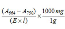
A664 = absorption at 664nm A750 = absorption at 750nm E = Extinction coefficient (100% acetone = 88.15, 90% acetone = 87.67) from Jefferies and Humphrey (1975) l = cuvette path length (cm) |
|
4.3. |
A series of dilutions using 90% acetone (N> 5) are then made and read, recording both Rb and Ra values. Blank values should be subtracted from the Rb and Ra prior to performing calculations. If using a fluorometer with multiple sensitivity and range settings such as a Turner model 10, then the proper blank value must be subtracted for readings taken at a given setting. |
|
4.4. |
A calibration factor (F) must be calculated for each fluorometer. It is the slope of the line resulting from plotting the fluorometer reading (x-axis) vs. chlorophyll concentration (y-axis). This line is forced through zero. An acidification coefficient (τ) is the average acid ratio (Rb/Ra) for the pure chlorophyll standards used in the calibration. |
|
4.5. |
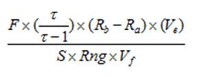
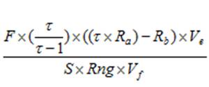
Calculating chlorophyll and phaeopigment concentration in a sample is accomplished by using the following equations (Knap et al., 1996):
Chl (µg/l) =
Phaeo (µg/l) = F = Linear calibration factor (see 4.4) τ = Average acid ratio (Rb/Ra) - Note that these are actually corrected values, with the blank readings already subtracted. Ve = Volume of extract (ml) Vf = Volume of sample filtered (l) S = Sensitivity setting of fluorometer (Applicable to Turner model 10. If using a model 10AU or another fluorometer, use a value of “1”) Rng = Range setting of fluorometer (Applicable to Turner model 10. If using a model 10AU or another fluorometer, use a value of “1”) There are variations of this equation that can be used and other factors that can affect chlorophyll measurements. More detailed descriptions can be obtained in Strickland and Parsons (1968) and Holm-Hansen and Riemann (1978).
Note: After a cruise, the fluorometer is calibrated again and the calibration factors and average acid ratios obtained from pre and post-cruise calibrations are averaged for final data processing. |
5. Reading Samples on the Fluorometer
|
5.1. |
The fluorometer should be allowed to warm up for approximately 1/2 hour before using it. Samples must extract in acetone for at least 24 hours prior to reading on the fluorometer and should be read before 48 hours. |
|
5.2. |
Samples must be at room temperature prior to reading. One hour before samples are to be read, they should be removed from the refrigerator and allowed to warm up in a dark place. |
|
5.3. |
A blank tube containing the same acetone batch used for the extractions should be prepared and read prior to reading samples. This blank should be read before and after every sample run and after door setting have been changed (Turner model 10 fluorometer) |
|
5.4. |
A coproporphyrin standard should be read prior to reading samples (D’Sa et al., 1997). While not used in any calculation, it is useful to monitor the performance of the fluorometer over time between calibrations. Significant changes in coproporphyrin readings may indicate a problem with the fluorometer. |
|
5.5. |
Remove the filter, shake the sample to insure that it is well mixed, and use a Kimwipe to remove fingerprints from the exterior of the tube prior to running samples. |
|
5.6. |
Read the sample and record the number (Rb). Add 100µl of 10% HCl and wait approximately 30 seconds for the number to stabilize and record the value (Ra). |
6. Equipment/Supplies
· Whatman 25mm GF/F filters (Fisher Scientific)
· Volumetric sample bottles (~130-150ml)
· Vacuum filtration apparatus with vacuum pump capable of maintaining 10 p.s.i
· Fluorometer and proper filter kit for measuring chlorophyll a/phaeophytin with acidification method (Turner model 10AU uses a 10-037R optical kit).
· Pipet (or re-pipet) capable of delivering 100µl.
· Personal protection equipment (PPE) consisting of gloves and safety glasses.
· Kimwipes or equivalent laboratory wipes.
· 10ml screw-top sample tubes (Fisher Scientific)
· Two sets of forceps (one for sample manipulation and one for replacing clean filters)
· Assorted laboratory glassware, including volumetric flasks for diluting calibration standards
7. Reagents
· Milli-Q or equivalent polished water source.
· HPLC-grade or equivalent low-fluorescing acetone. Note that volume is not conserved when preparing solution of water and acetone. The addition of 413ml Milli-Q water to 3800ml of acetone results in 4130ml of 90% acetone.
· 10% HCl solution
· Chlorophyll a (Sigma Aldrich catalog number C6144)
· Coproporphyrin III tetramethyl ester (Sigma Aldrich catalog number C7157)
8. References
· D’Sa, E.J., Lohrenz, S.E, Asper, V.L., and Walters, R.A. (1997). Time Series Measurements of Chlorophyll Fluorescence in the Oceanic Bottom Boundary Layer with a Multisensor Fiber-Optic Fluorometer. , 167: 889–896. DOI: 10.1175/1520-0426(1997)0142.0.CO;2
· Holm_Hansen, O., Lorenzen, C.J., Holms, R.W., Strickland, J.D.H. (1965). Fluorometric Determination of Chlorophyll. J. Cons.perm.int Explor. Mer. 30: 3-15.
· Holm-Hansen, O., and B. Riemann. (1978). Chlorophyll a determination: improvements in methodology. Oikos, 30: 438-447.
· Jeffery, S.W. and Humphrey, G.F. (1975). New spectrophotometric equations for determining chlorophylls a, b, c1, and c2 in higher plants, algae and natural phytoplankton. Biochem. Physiol. Pflanz. 167: 191-194.
· Knap, A., A. Michaels, A. Close, H. Ducklow and A. Dickson (eds.). (1996). Protocols for the Joint Global Ocean Flux Study (JGOFS) Core Measurements.
JGOFS Report Nr. 19, vi+170 pp. Reprint of the IOC Manuals and Guides No. 29, UNESCO 1994.
· Lorenzen, C. J. (1967) Determination of chlorophylls and phaeopigments: spectrophotometric equations. Limnol. Oceanogr. 12: 343–346.
· Strickland J. D. H., Parsons T. R., (1968). A practical handbook of seawater analysis. Pigment analysis, Bull. Fish. Res. Bd. Canada, 167.
· Yentsch, C.S., Menzel, D.W. (1963). A method for the determination of phytoplankton chlorophyll and phaeophytin by fluorescence. Deep-Sea Res. 10: 221-231
Prior to CalCOFI's use of Guildline's Autosal and Portasal, different instrumentation or techniques were used to measure seawater sample salinities. When I first participated in cruises in the mid-1980's, salinities were collected in 250ml sample bottles with wire bail ceramic stoppers with rubber washer. These samples were run on a Plessey (Hytech) Laboratory Salinometer. I went online to find out more about this particular instrument for our instrumentation timeline and was surprised at how little I found. Fortunately, I have a photocopy of the original Hytech manual so I scanned it to PDF. (JRW 06/2019)
In 1970, this salinometer was relabeled Plessey Model 6230 Portable Laboratory Salinometer by Plessey Environmental Systems.
("In 1970, Bissett-Berman was purchased by the British company Plessey Ltd. and the San Diego Division was renamed Plessey Environmental Systems. Ten years
later, Grundy bought the parent company of Plessey Environmental and a short time later phased out the oceanographic equipment.")
| Salinity Sample bottle similar to what was used by CalCOFI in 1970-1990 |
Plessey/Hytech Laboratory Salinometer Model 6220 Manual (click for PDF of photocopy) |
.jpg) |
 |
CTD General Practices: System Description, Deployment, Data Aquisition, & Maintenance
SUMMARY: Since 1993, the CalCOFI program has deployed a Seabird 911 CTD mounted on a 24-bottle rosette during seasonal, quarterly cruises off California. The CTD-rosette is lowered into the ocean to 515m, depth-permitting, on 75 hydrographic stations using the ship's conductive-wire winch. Data from the sensors are transmitted up the conductive wire and displayed real-time on a data acquistion computer. Discrete seawater samples are collected in 10L bottles at specific depths determined by the chlorophyll maximum and mixed layer depth. These samples are analyzed at sea and used to assess the CTD sensor data quality plus measure additional properties. Processed CTD sensor data are compared to the seawater sample data and corrected when necessary. Preliminary data are available on CalCOFI's website, calcofi.com, while the cruise is at sea when internet is available. Preliminary processed data files are online shortly after the cruise returns. Final, publication-quality bottle & CTD data are available once the bottle data have been fully processed & scrutinized.
1. Basic CTD Components
The Seabird 911/911plus CTD configuration has evolved since 1993. Components are added or upgraded as new sensor technology becomes available.
The current (since Nov 2009) CTD & sensors configuration:
- SBE9plus CTD with SBE11 v2 Deck Unit (CTD 911plus); rated to 6800m
- dual SBE3plus fast response temperature sensors (T); rated to 6800m
- dual SBE4C conductivity sensors (C); rated to 6800m
- dual SBE43 oxygen sensors (O2); rated to 7000m
- dual SBE5T pumps; rated to 10,500m
- Seapoint Chlorophyll Fluorometer; passive flow (not pumped), mounted on rosette, not shuttered; rated to 6000m
- Wetlabs C-Star Transmissometer; 25cm 660nm, passive flow; rated to 6000m
- Satlantic ISUS Nitrate sensor; since 0411; v1 ISUS powered by an external 12v battery, passive flow; rated to 1000m
- Seabird SBE-18 pH sensor; since 0911; rated to 1200m
- Datasonics/Teledyne-Benthos PSA-916 Altimeter; mounted unobstructed & low; rated to 6000m
- Biospherical Remote Photoradiometer (PAR) QSP-2300; rated to 2000m; alternate model QSP-200L; rated to 1000m
- Biospherical Surface Photoradiometer (PAR) QSR-240; attached to deck unit
- Remote Depth Readout SBE14; attached to deck unit; allows winch operator to see CTD depth
2. Preparation & Deployment
Weather-permitting, the CTD and bottles are prepared for deployment 20 minutes prior to station arrival.
CTD-rosette preparations on CalCOFI cruises include:
- Prep the electronics: removal of fresh-water rinse tubes attached to the pumps; removal of the PAR protective cap;removal of the pH sensor cap; RBS rinse (using a squirt bottle) the transmissometer lenses to eliminate surface film.
- Prep the rosette bottles: 24-10 liter bottles are propped open by stretching the spring-loaded end caps back and securing their nylon lanyards to the proper carousel position. Bottle breathers & sample-drawing valves are checked for closure. Tag lines are attached to the rosette and once secured, the deck straps are removed. ISUS nitrate sensor battery deck charging cable is disconnected and set out of the way and the battery connected to the sensor.
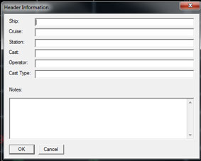
- Electronics warmup: after bottle prep, ~fifteen minutes prior to station arrival, the CTD deck unit is turned on, powering up the CTD electronics. Seabird has recommended at least a 10min warmup to improve SBE43 oxygen data at surface. After filling out the header form (see example), data aquisition is started. The ISUS nitrate sensors power cable is attached to the battery to allow several minutes warmup prior to deployment if not done after bottle prep.
- Before deployment, the CTD's pressure reading on-deck is logged on the console ops form. This value is monitored at the beginning and end of the cast for shifts in the pressure baseline. It's median on-deck reading should be ~0. If the on-deck pressure become greater than +-0.3db, a corrective pressure sensor offset should be applied and documented in the CTD cast notes. It is important to wait several minutes after turning on the CTD deck unit before assessing the deck pressure.
- The CTD-rosette is launched and held just below surface; enough wire is paid out so the bottle tops do not break surface when the ship rolls. SIO-CalCOFI uses high visibility yellow tape above the cable grip as a visual guide for the winch operator to adjust 0m.
- The winch readout is zeroed and the CTD is sent to 10 meters for ~2 minutes to purge air from the system, allow the pumps to turn on (triggered by seawater contact; status is verified on the CTD computer screen). This gives the sensors a few minutes to stabilize and thermally equilibrate after sitting on-deck. (Please note that some CTD operators do not power-up the CTD system until the unit is in the water. This a a precaution recommended by some programs and UNOLS but not practiced by SIO-CalCOFI. Since 1990, SIO-CalCOFI has powered up the system on-deck then deployed and never had a problem.)
- Communicating with the winch operator using intercom or radio, the CTD operator requests the CTD return to just below surface. Data archiving is initialted by selecting Real-Time Data/Start Archiving in Seasave (IMPORTANT if data archiving has not already started) and Display/Erase All Plots clears the surface & 10m soak noisy plots. Hold at surface for ~one minute to log data and verify T, C, & O2 sensor correctness & agreement between the primary and secondary pairs.
- If everything looks good, the CTD is lowered to 515m, depth-permitting, at 30m/min for the first 100m then 60m/min to terminal depth.
- If the bottom depth is less than 515m, the CTD is lowered to 10m above the bottom, according to the altimeter reading, not wire readout. After the wire settles and if conditions permit, the CTD depth may be adjusted to ~5m above the bottom if a standard level is attainable.
3. Data Acquistion & Seawater Collection
Our CTD data acquistion system is a Intel (ASUS) blade PC running Windows 7 64-bit and Seasave v7, Seabird's data acquisiton program. Calibration coefficients for each sensor are entered during CTD setup and termination before the first cast. Data are logged at 24hz to insure maximum resolution & flexibility in post-cast data processing; 24Hz data allow re-calculation of derived values using different post-cast or post-cruise coefficients. The SBE11 deck unit v1 auto-applies a 0.073ms offset to the primary conductivity only. The SBE11 deck unit v2, used since Jul 2009, auto-applies a 0.073ms offset to both primary & secondary conductivity sensors.
During the cast, Seasave's main plot window displays real-time temperature, salinity, oxygen, and fluorometry versus depth. Seasave has a 4 parameters-per-plot limitation so additional plots are used to display other sensor profiles. A fixed-data window lists real-time data in numeric form so T, C, & S values may be transcribed to the CTD console operations log prior to bottle closure.
- When the CTD arrives to the target depth, time, wire out, depth, T, C, S, & alt (if near bottom) are written on the console ops form. This usually takes at least 20secs, the minimum mandated flushing time before closing a bottle.
- In Seasave, the 'create marker' command is initiated followed by the 'fire bottle' command. When the bottle closure confirmation is received by the deck unit, the 'bottles fired' will increment by one. The CTD operator records the confirmation time on the bottle depth record, then checkmarks the bottle confirmation boxes.
- When the first bottle has closed, the bottle-closure confirmation time, latitude, longitude, and bottom depth (from echo sounder), are recorded on the form's CTD-At-Depth sidebar. If a cruise event log is running, a CTD AT DEPTH event is logged. A 500m CTD cast takes ~50mins so the GPS position & time recorded during the first bottle trip becomes the primary cast information for the bottle data.
- The CTD-rosette is raised to the next target bottle depth at ~60m/min, conditons permitting. Console ops logging and bottle closure steps (1 & 2) are repeated until the CTD-rosette is back at surface and final bottle closed.
- The CTD-rosette is recovered using taglines and once on deck, re-secured to the deck eyes with short lines or strap.
- The deck pressure is recorded on the console ops form and data aquisition is halted.
- SIO-CalCOFI-authored CTD backup program (CTDbackup.exe) is used to immediately zip all cast files and archive the zip file to other media. This program also generates an electronic sample log using the CTD AT DEPTH event plus .hdr & .mrk files to log seawater samples (see CESL: CalCOFI Electronic Sample Log).
- The ISUS power cable is disconnected, PAR & pH sensors are capped.
4. Water Sampling
Seawater samples are drawn from the 10L rosette bottles once the CTD-rosette has been secured. Oxygen samples are drawn first, followed by DIC/pHs, salts, nutrients, chlorophylls (from depths 200m or less), and LTER's suite of samples. Please refer to the specific water sampling or analytical method for more information.
5. Quality Control
The CTD electronics and sensors are reliable and stable when properly serviced and maintained. CalCOFI has established some standard practices over time to keep the CTD functioning properly.
- De-ionized or freshwater rinses: post-cast the plumbed-pumped sensors (2 pairs of T, C, O2, & pump) are flushed with de-ionized or Milli-Q water to minimize bio-fouling.
- The carousel is hosed with fresh water to reduce mis-trips from bio-fouling or inorganic particulate buildup. A vinyl rosette cover is used when the CTD-rosette needs protection from contaminants or debris.
- PAR and pH sensor (stored in buffer) are capped when on-deck.
- Deck tests are performed before the first cast to derive transmissometer coefficients based on in-air and blocked light path voltage readings. A chlorophyll standard, finger or palm (yes - your finger or hand can be used max out the fluorometer, just avoid touching the optical surfaces) in front of the fluorometer optics can test the maximum response voltage. Deck tests are performed occasionally during the cruise to monitor transmissometer and fluorometer stability and response.
- At-sea analyses of seawater samples allow bottle data to be compared to sensor data quickly, particularly salinities. When bottle salts are analyzed, the bottle salinity calculation is immediately compared to the CTD value and flagged if significantly different. This allows early detection of analytical equipment or CTD sensor malfunction. Oxygen, chlorophyll, and nutrients data comparisons are less immediate but when data look suspect, this ability helps identify real vs faulty measurements. Oxygen sample draw temperature (temperature of the seawater sample at the time the O2 sample is taken) is the first indicator of bottle mistrip. If the O2 draw temperature does not follow the trend indicated by the CTD temperture displayed on the sample log. The bottle may have closed at the wrong depth.
6. Equipment/Supplies
Conditions at sea can be rough and gear can break so CalCOFI prefers to have backups of all mission-critical components to conserve shiptime. Replacing defective gear often takes less time then troubleshooting or repairs. All sensors include their respective sensor-to-CTD interface cables plus spares.- 2 - Seabird SBE9plus CTDs with sensors; the primary package is inventoried in section 1; sensors without backups: ISUS nitrate sensor, pH sensor, deck unit remote depth readout
- 2 - deck units: primary SBE11v2; backup SBE11v1
- 2 - Windows 7 (ASUS blade) computers with 2 serial ports; deck unit, & GPS interface cables.
- 2 - SBE32 carousels; plus spare trigger assemblies
- Console operations forms plus clipboard
- Timer, for 2 minute soak at surface
- 2 - 24 place aluminum rosette frame
- 2 - sets of 24 10L Niskin bottles; plus 4 spare bottles; multitude of spare parts
- 2 - sets of 24 nylon lanyards for Niskin bottles
- Termination toolkit and supplies - please refer to termination documentation for info on CalCOFI CTD wire termination techniques.
- butane soldering wand, solder, butane
- adhesive-lined shrink tubing: 1/8"
- Scotch 130 electrical splicing tape
- Scotch 33 electrical tape
- Scotch-kote electrical coating
- Cable grips, stainless steel thimbles, and shackles to attached sea cable to the rosette
- 3 - taglines with detachable hooks
- 3 - 1m deck lines to secure the rosette on deck; straps
- 4L Milli-Q filled carbuoy with hose for flushing the plumbed sensors post-cast
- Hose, for freshwater rinse of carousel and other components post-cast
- Stainless steel hose clamps: 100 - size 88 for mounting Niskin bottles to the rosette; misc others to mounted the CTD, ISUS, battery, and sensors to the frame.
Turner Designs fluorometer standard for SCUFA (fits Seapoint fluorometer) for deck calibration;Black rubber "card" for transmissometer deck test. Currently we using Wetlabs ECO-Fl fluorometer which does not have an optical path that works with the Turner Designs standard so fingers an inch away from the detector is used to max out the voltage. Seapoint flurometer is backup.- RBS or Micro in a squirt bottle for rinsing the transmissometer lenses before deployment. RBS or Micro are residue-free soaps in dilute Milli-Q solutions.
- CTD cable servicing kit containing silicone grease; electrical contact cleaner; cotton swabs; Kim-wipes
- 3 - Wetlabs 12v batteries, multi-battery charging station, on-deck weather-proof battery charging cable for ISUS nitrate sensor batteries.
7. Maintenance
CalCOFI sends all CTD electronics to their respective manufacturer for service and maintenance. The conductivity, and oxygen sensors are serviced & re-calibrated after use on two consecutive cruises (~150-200 deployments). SBE3plus temperature sensor calibration has changed to annually since the stability of these sensors is well documented. Routine Seabird carousel maintainance is performed by the CalCOFI-SIO Technical Group (CSTG). When repairs or five-year service are needed, the carousel is sent to Seabird. PAR sensors are serviced by Biospherical every three years.
General protocol is any sensor is returned for repair if the sensor fails or data quality diminishes. The SBE9+ CTD ('fish') is routinely serviced every five years. The aluminum-frame rosette is repaired or modified at SIO's Research Support Shop whenever necessary.
8. References
- Sea-Bird Electronics, Inc, 2009. SBE 9plus Underwater Unit Users Manual, Version 012
- Sea-Bird Electronics, Inc, 2009. SBE 11plus V2 Deck Unit Users Manual, Version 012
- Sea-Bird Electronics, Inc, 1998. SBE 32 Carousel Water Sampler Operating and Maintenance Manual
Subcategories
CalCOFI Handbook
The CalCOFI Handbook is a compilation of information for cruise participants. It explains many aspects of the science performed at sea, particularly the sample drawing methods for each sample type.
Data Formats
CalCOFI Data File Formats
Methods
CalCOFI standard practices for sample analysis, data processing, metadata & general methodology.
Software
SIO-CalCOFI software used at-sea and ashore, developed by the SIO CalCOFI Technical Group. Plus other software: auto-titrator oxygen analysis software developed by SIO's Ocean Data Facility; Seabird Seasoft & Data Processing software; Microsoft Office, Ultraedit, Ztree, hxD hex editor, Matlab, Surfer, Ocean Data View.